EKIO Theme
theme_ekio() applies EKIO’s visual identity to any
ggplot2 plot. It builds on theme_minimal() with curated
typography, spacing, and color choices.
ggplot(mtcars, aes(wt, mpg)) +
  geom_point(color = ekio_pal("blue")["700"], size = 2.5) +
  labs(
    title = "Fuel Efficiency vs. Weight",
    subtitle = "Motor Trend Car Road Tests (1974)",
    x = "Weight (1000 lbs)",
    y = "Miles per Gallon"
  ) +
  theme_ekio()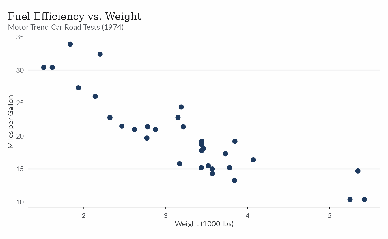
The grid parameter controls which major grid lines are
drawn:
ggplot(mtcars, aes(wt, mpg)) +
  geom_point(color = ekio_pal("blue")["700"]) +
  theme_ekio(grid = "xy")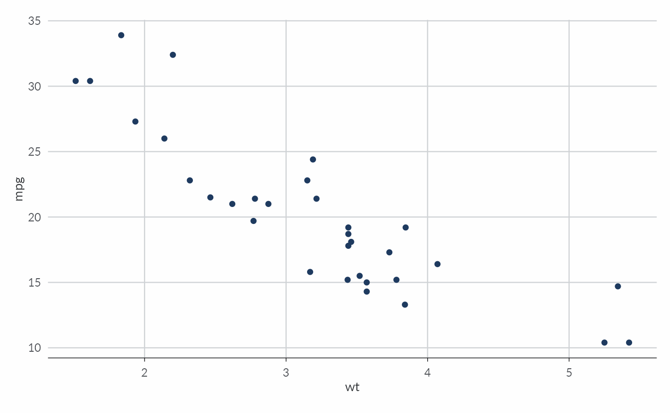
Plot surfaces
theme_ekio() supports three named surfaces: the default
warm off-white, "white", and the cool white
"cold". You can also supply a hex color.
ekio_surface() resolves a named surface to its hex code for
use elsewhere.
ekio_surface("cold")
#> [1] "#F6F7F8"

ggplot(mtcars, aes(wt, mpg)) +
  geom_point(color = ekio_pal("blue")["700"], size = 2.5) +
  theme_ekio(background = "#F6F7F8")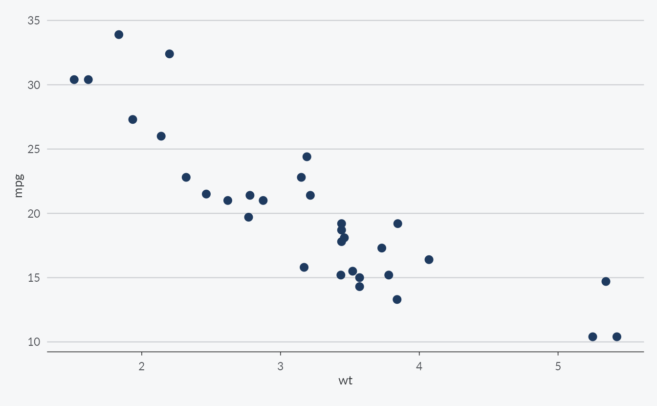
Color Palettes
ekioplot ships 28 palettes across seven groups. Use
list_ekio_palettes() to explore them:
str(list_ekio_palettes())
#> List of 7
#>  $ accent     : chr [1:3] "gold" "accent_blue" "accent_orange"
#>  $ brand      : chr "ekio_brand"
#>  $ academy    : chr [1:2] "yoro_blue" "yoro_green"
#>  $ categorical: chr [1:6] "full" "full_muted" "full_light" "spectrum_light" ...
#>  $ sequential : chr [1:8] "blue" "gray" "stone" "teal" ...
#>  $ diverging  : chr [1:4] "purple_orange" "blue_red" "teal_orange" "purple_green"
#>  $ scientific : chr [1:4] "okabe_ito" "viridis" "inferno" "plasma"
Access any palette with ekio_pal():
ekio_pal("full")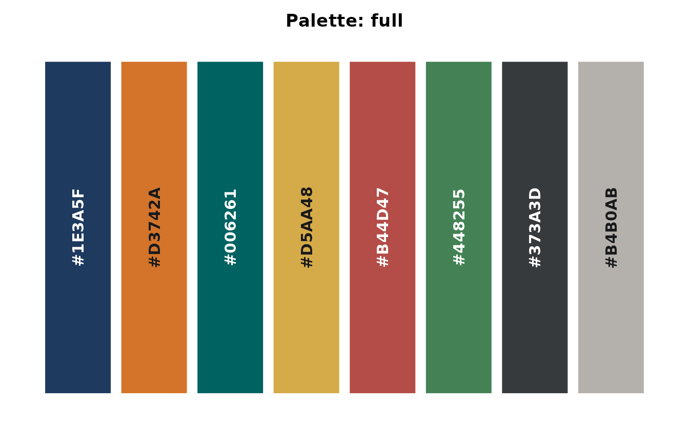
ekio_pal("cool3")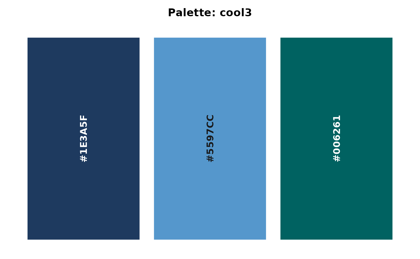
ekio_pal("accent_blue", n = 5)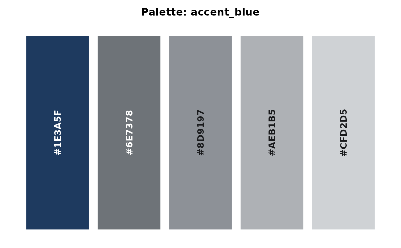
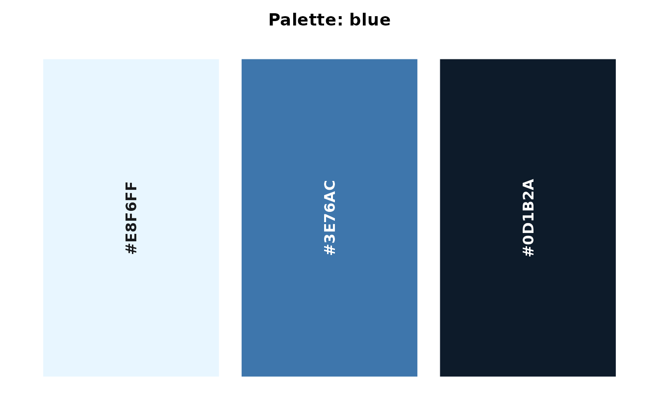
ekio_pal("blue", n = 5)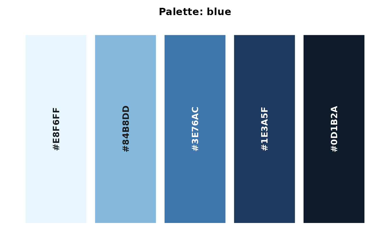
Palette types
-
Categorical:
full,full_muted,full_light,spectrum_light,cool3,cool4 -
Brand:
ekio_brandfor EKIO identity assets, not general data visualization -
Academy:
yoro_blue,yoro_greenfor EKIO Academy tutorials and books -
Scientific:
okabe_ito,viridis,inferno,plasma -
Sequential:
blue,gray,stone,teal,green,orange,red,purple -
Accent:
gold,accent_blue,accent_orange -
Diverging:
purple_orange,blue_red,teal_orange,purple_green
accent_blue and accent_orange return four
colors by default. Set n from 2 to 6 to match the number of
series while retaining the accent as the first color. gold
remains a fixed three-color named palette.
ekio_pal() displays a swatch when printed:
ekio_pal("full")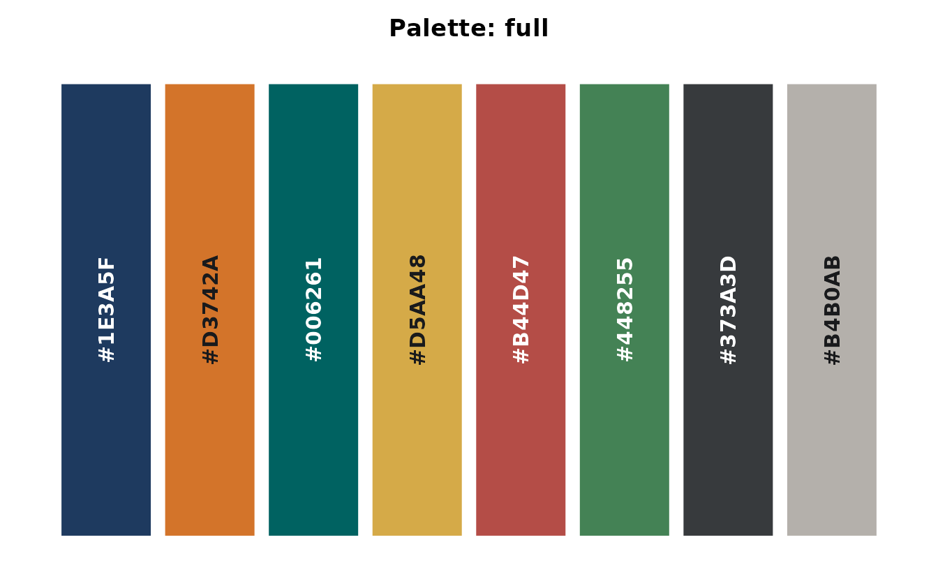
Scale Functions
ekioplot provides ggplot2 scales for both discrete and continuous data.
Discrete scales
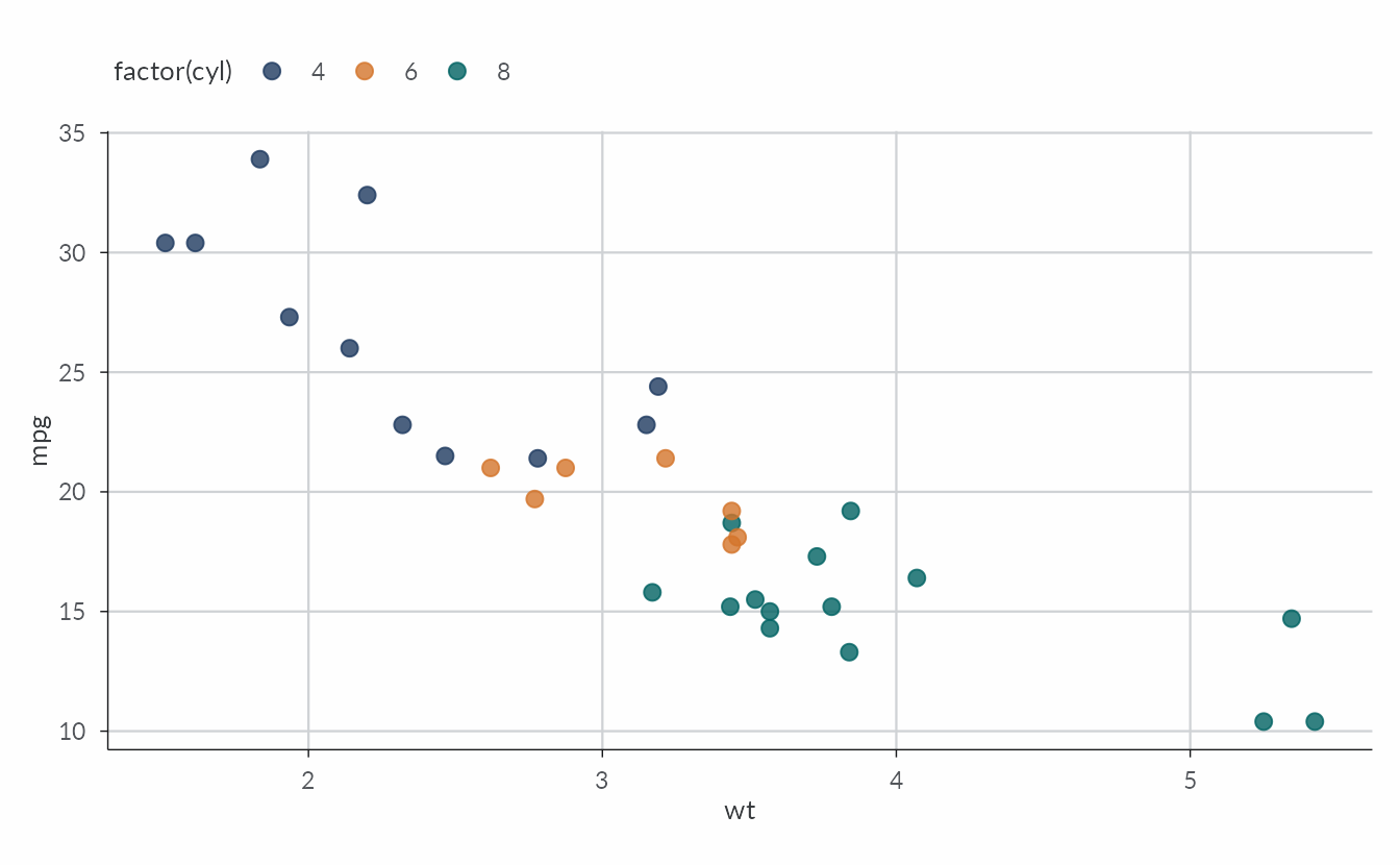
ggplot(mtcars, aes(wt, mpg, color = factor(cyl))) +
  geom_point(size = 3) +
  scale_color_ekio_d("full") +
  labs(color = "Cylinders") +
  theme_ekio(grid = "xy")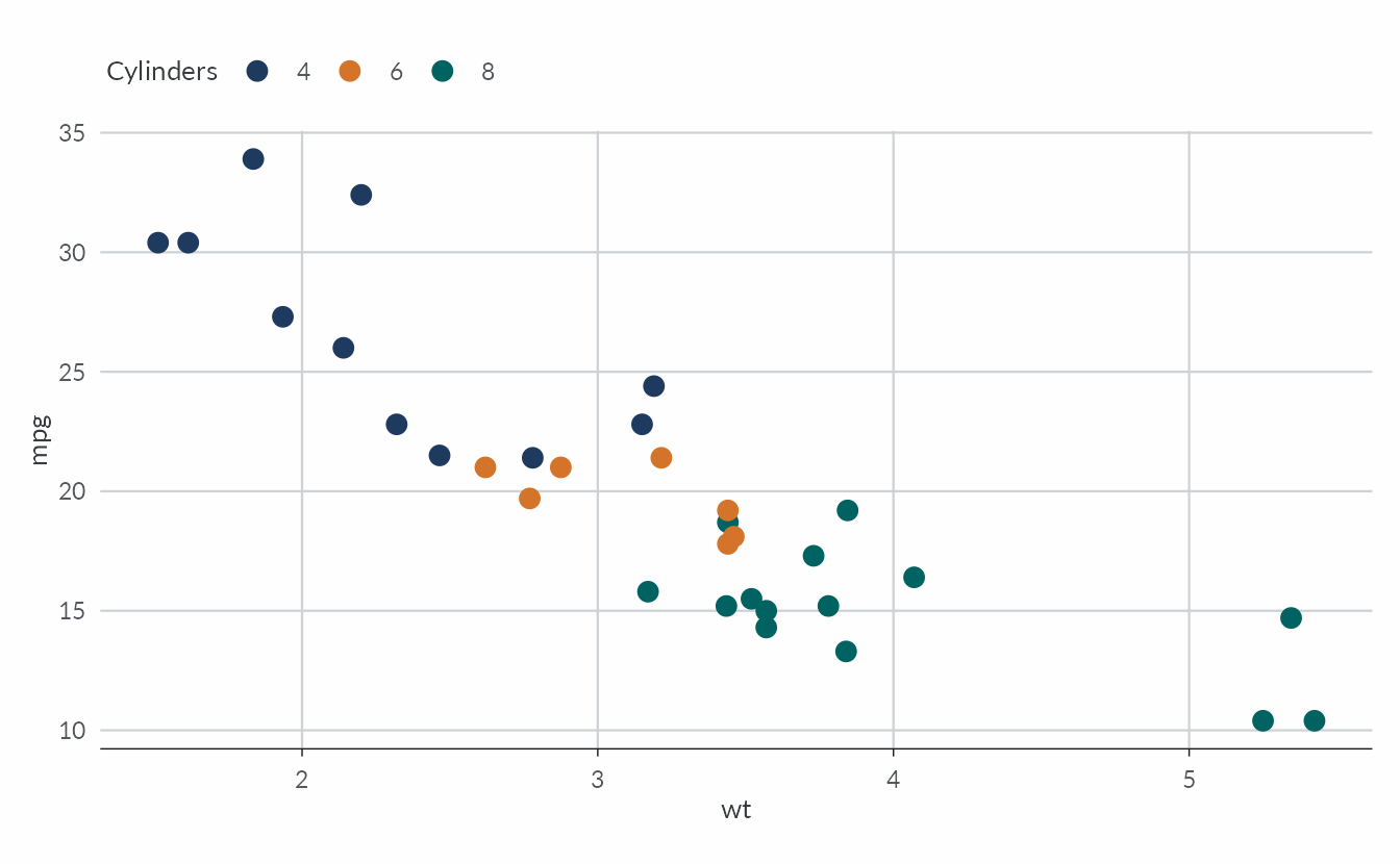
Continuous scales
Sequential and diverging palettes work with continuous data:
ggplot(mtcars, aes(wt, mpg, color = hp)) +
  geom_point(size = 3) +
  scale_color_ekio_c("blue") +
  labs(color = "Horsepower") +
  theme_ekio(grid = "xy")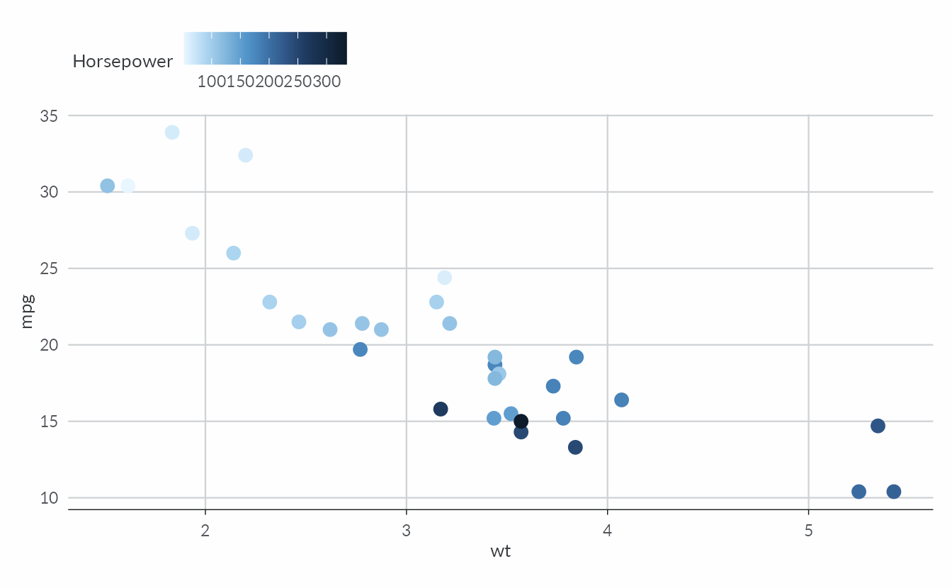
Fill variants are available as scale_fill_ekio_d() and
scale_fill_ekio_c().
Recipe Functions
Recipe functions are high-level wrappers that create complete, publication-ready plots with smart defaults.
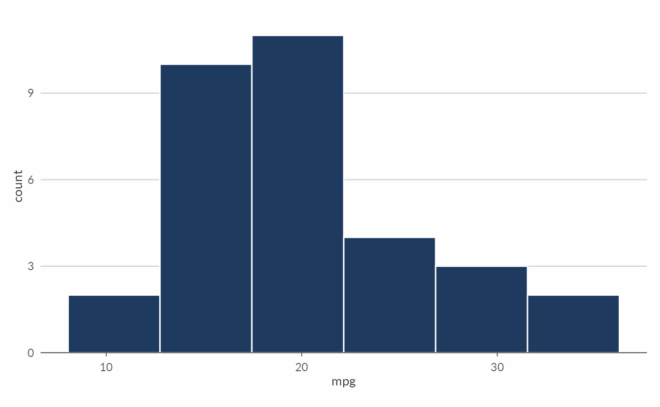
Bar plot
cyl_counts <- as.data.frame(table(cyl = mtcars$cyl))
names(cyl_counts)[2] <- "n"
ekio_barplot(cyl_counts, cyl, n)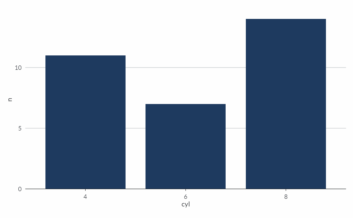
Area plot
economic_series <- subset(
  ggplot2::economics_long,
  variable %in% c("pce", "psavert", "uempmed")
)
ekio_areaplot(economic_series, date, value01, fill = variable)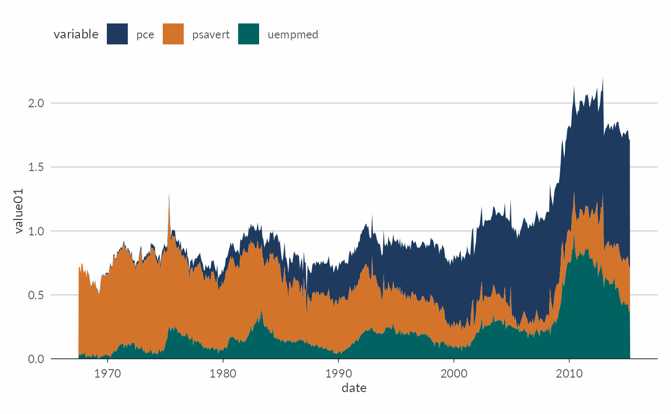
Smart aesthetic detection
Recipe functions automatically detect whether the color/fill argument is:
- Missing — uses EKIO blue as default
-
A color string (e.g.,
"steelblue") — uses that color directly - A variable — maps it and applies the appropriate EKIO scale
ekio_histogram(mtcars, mpg, fill = "coral")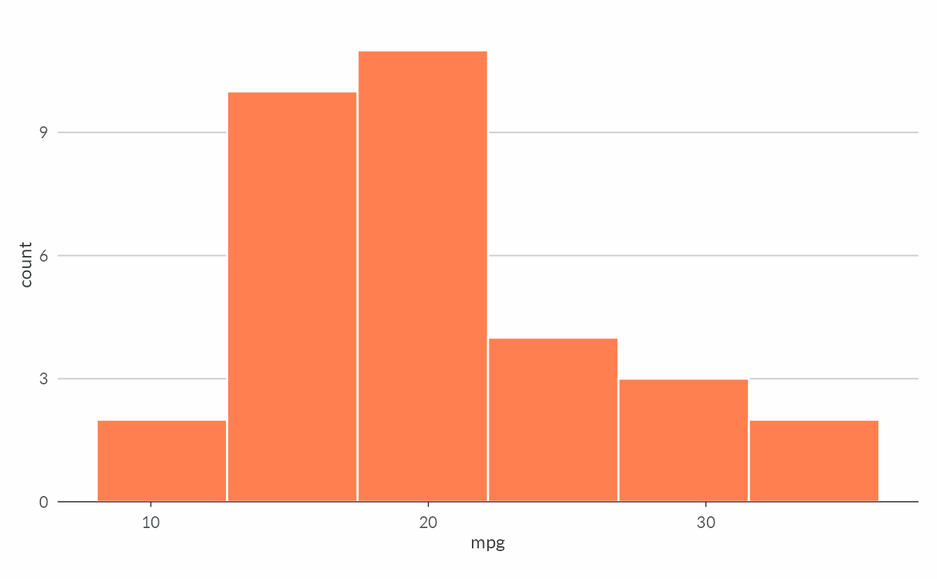
Brand Scales
Every brand color is reached through ekio_pal(). The
brand scales — "blue", "gray",
"stone", "teal", "green",
"orange", "red", and "purple" —
are nine-step ramps running light to dark, named by shade. All sit on
one lightness spine, so a given shade carries the same visual weight in
every family:
ekio_pal("gray")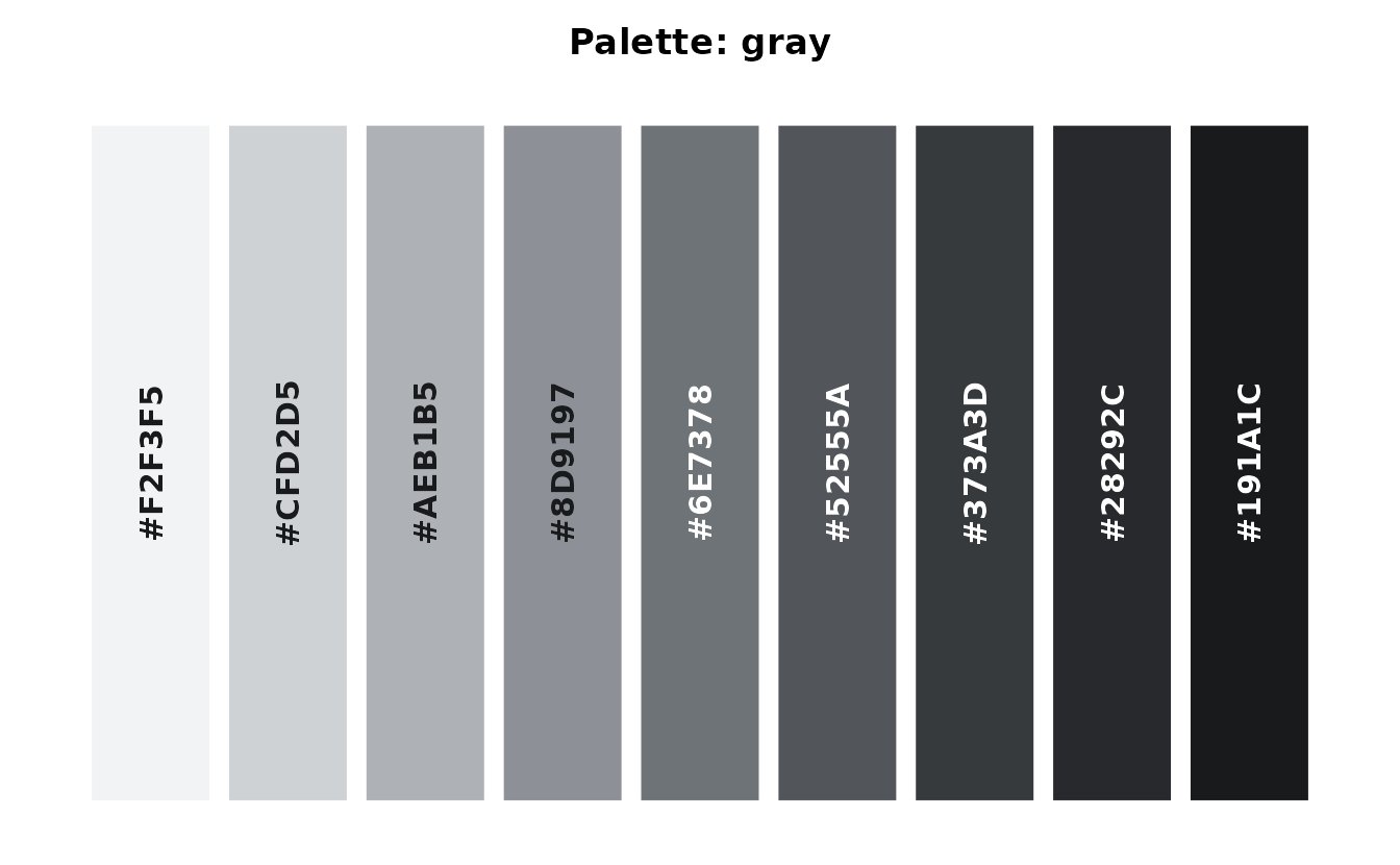
Position and shade are aligned by construction, so element
i is always shade i * 100. Index whichever way
reads better:
Because these are the same objects used for continuous fills, asking for fewer colors interpolates across the whole ramp rather than returning the lightest few:
ekio_pal("blue", n = 3)