Detrending Series

The trend extraction methods covered in the other vignettes return a smooth trend. Often, though, the trend is exactly the part we want to remove: in macroeconomics the object of interest is usually the deviation from trend — the cycle, or the output gap when the series measures aggregate activity. detrend_series() removes the trend from a series and adds the detrended series as a column to the original data frame.

library(trendseries)
library(dplyr)
library(tidyr)

The theme below is used throughout the vignette for consistent styling.

library(ggplot2)

theme_series <- theme_minimal(paper = "#fefefe") +
  theme(
    legend.position = "bottom",
    panel.grid.minor = element_blank(),
    strip.background = element_rect(fill = "#2c3e50"),
    strip.text = element_text(color = "#fefefe"),
    axis.ticks.x = element_line(color = "gray40", linewidth = 0.5),
    axis.line.x = element_line(color = "gray40", linewidth = 0.5),
    axis.title.x = element_blank(),
    palette.colour.discrete = c(
      "#2c3e50",
      "#e74c3c",
      "#f39c12",
      "#1abc9c",
      "#9b59b6"
    )
  )

Trend extraction vs detrending

detrend_series() is the mirror image of augment_trends().

augment_trends() returns the trend (trend_* columns) and discards the fluctuations around it.
detrend_series() returns the fluctuations (detrend_* columns): the trend is fitted with the same methods and then subtracted from the series, so value = trend + detrend.

Any trend method supported by augment_trends() can be used for detrending. The default is the Hodrick-Prescott filter ("hp"), a conventional detrending choice for economic data, with the smoothing parameter set automatically from the frequency of the series. And unlike decompose_series(), which needs a seasonal component to isolate, detrending is well defined at any frequency.

A first detrended series

Let’s start with the ibcbr dataset, a monthly index of Brazilian economic activity (IBC-Br) compiled by the Central Bank.

ggplot(ibcbr, aes(date, index)) +
  geom_line(lwd = 0.7) +
  scale_x_date(date_breaks = "2 years", date_labels = "%Y") +
  labs(
    title = "Brazilian economic activity (IBC-Br)",
    y = "Index (2003 = 100)"
  ) +
  theme_series

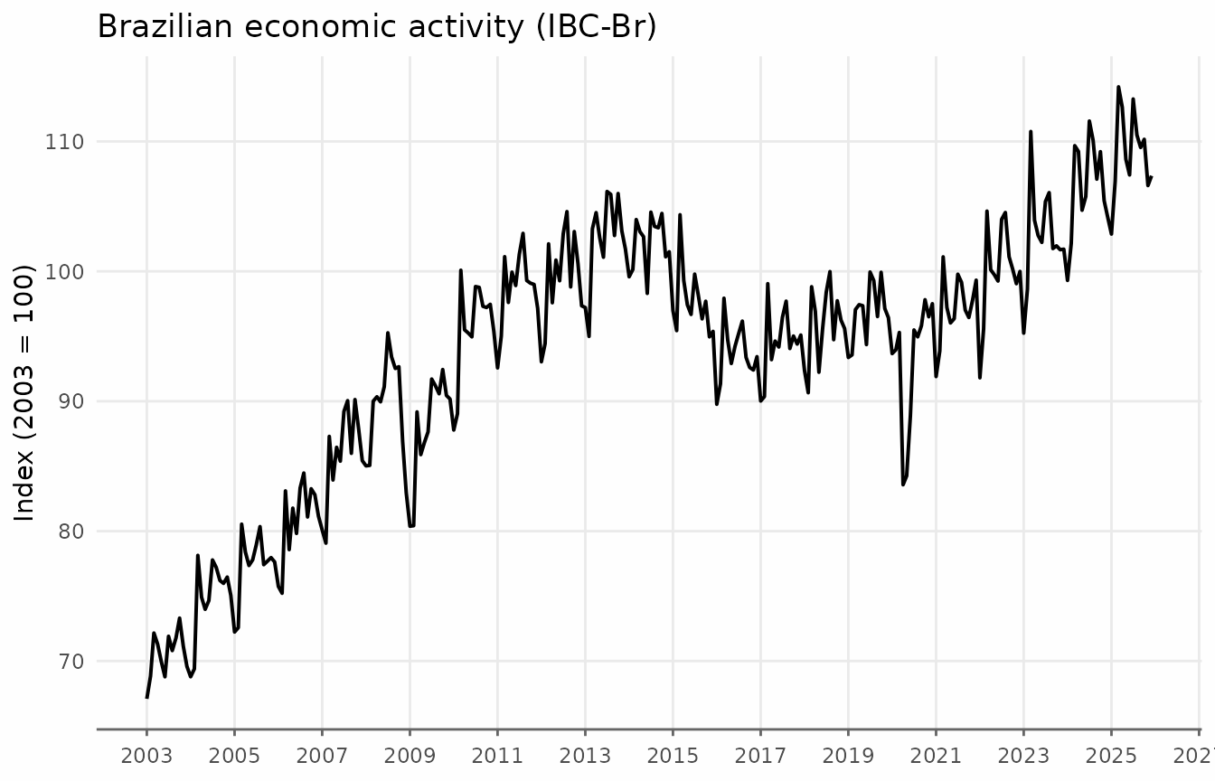
Passing the data to detrend_series() adds a single new column, detrend_hp, holding the deviation from the HP trend. The frequency is detected automatically from the date column.

ibcbr_cycle <- ibcbr |>
  detrend_series(value_col = "index")

ibcbr_cycle
#> # A tibble: 276 × 3
#>    date       index detrend_hp
#>    <date>     <dbl>      <dbl>
#>  1 2003-01-01  67.1     -1.93 
#>  2 2003-02-01  68.8     -0.482
#>  3 2003-03-01  72.2      2.53 
#>  4 2003-04-01  71.3      1.37 
#>  5 2003-05-01  70.0     -0.250
#>  6 2003-06-01  68.8     -1.75 
#>  7 2003-07-01  71.9      1.07 
#>  8 2003-08-01  70.8     -0.332
#>  9 2003-09-01  71.8      0.344
#> 10 2003-10-01  73.3      1.57 
#> # ℹ 266 more rows

ggplot(ibcbr_cycle, aes(date, detrend_hp)) +
  geom_hline(yintercept = 0, color = "gray40", lty = 2) +
  geom_line(lwd = 0.7) +
  scale_x_date(date_breaks = "2 years", date_labels = "%Y") +
  labs(
    title = "Detrended economic activity",
    subtitle = "Deviation from the HP trend",
    y = "Index points"
  ) +
  theme_series

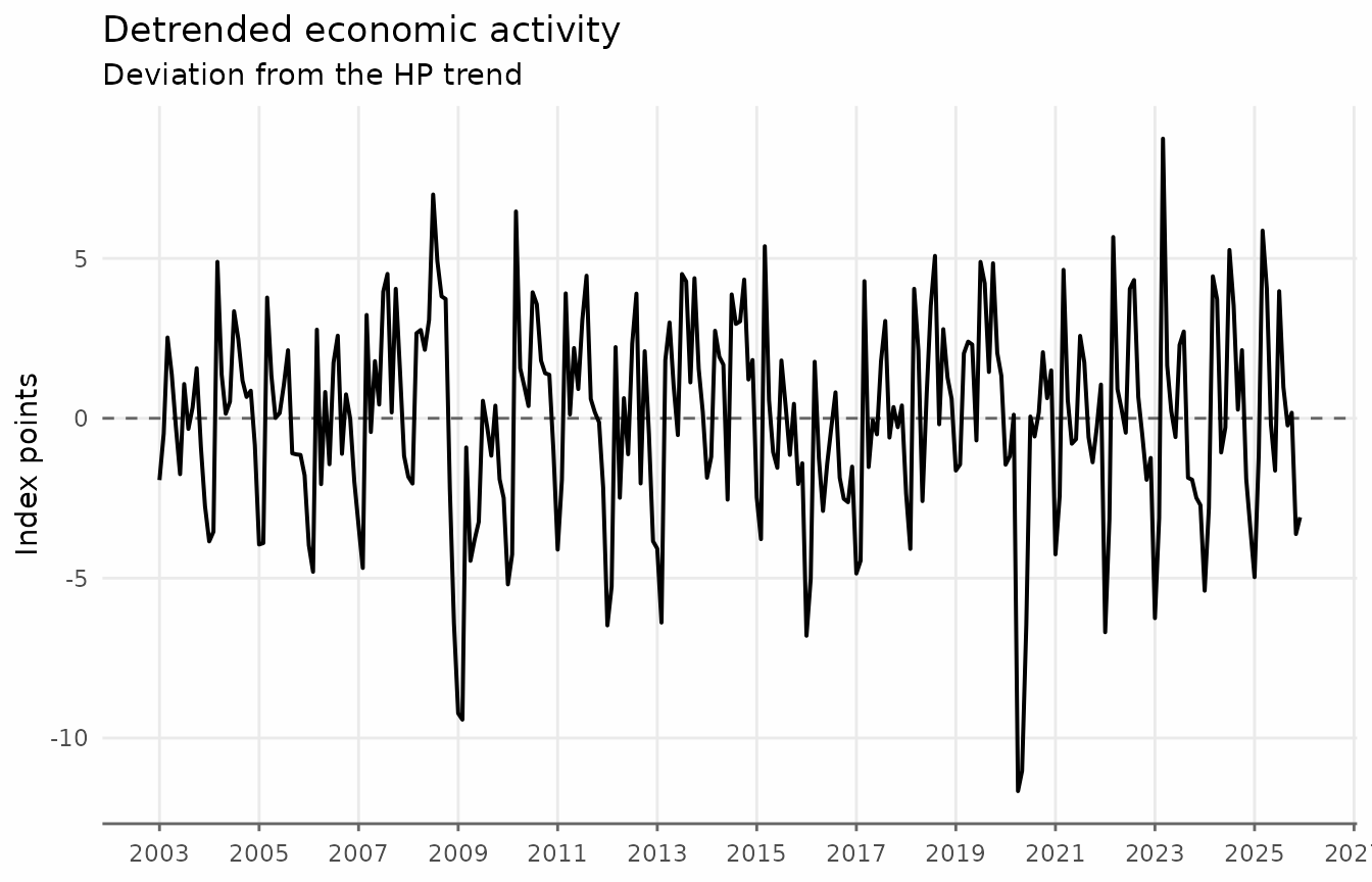
The big picture is fairly correct: the 2008–09 recession, the 2015–16 crisis, and the COVID collapse all show as deep negative deviations. But the line is also covered in a regular saw-tooth pattern. That isn’t the business cycle: it’s seasonality, and it points to an important caveat.

Detrending does not deseasonalize

The IBC-Br index above is not seasonally adjusted, and detrending only removes the slow-moving part of the series. The seasonal swings are too fast for the trend to absorb, so they end up in the detrended series.

The fix is to remove the seasonal component first, with deseason_series() and detrend the seasonally adjusted series. The two wrappers compose naturally: deseason_series() adds a seasadj_stl column, which detrend_series() can then take as its input.

ibcbr_sa_cycle <- ibcbr |>
  deseason_series(value_col = "index") |>
  detrend_series(value_col = "seasadj_stl")

ibcbr_sa_cycle
#> # A tibble: 276 × 4
#>    date       index seasadj_stl detrend_hp
#>    <date>     <dbl>       <dbl>      <dbl>
#>  1 2003-01-01  67.1        71.4     2.00  
#>  2 2003-02-01  68.8        72.5     2.77  
#>  3 2003-03-01  72.2        68.7    -1.30  
#>  4 2003-04-01  71.3        71.1     0.918 
#>  5 2003-05-01  70.0        70.5    -0.0433
#>  6 2003-06-01  68.8        69.6    -1.16  
#>  7 2003-07-01  71.9        69.0    -2.06  
#>  8 2003-08-01  70.8        68.1    -3.26  
#>  9 2003-09-01  71.8        71.6    -0.0420
#> 10 2003-10-01  73.3        72.0     0.0601
#> # ℹ 266 more rows

We can compare the approaches side by side.

cycles <- bind_rows(
  list(
    "Raw series" = ibcbr_cycle,
    "Seasonally adjusted" = ibcbr_sa_cycle
  ),
  .id = "input"
)

cycles <- cycles |>
  rename(cycle = detrend_hp)

ggplot(cycles, aes(date, cycle)) +
  geom_hline(yintercept = 0, color = "gray40", lty = 2) +
  geom_line(aes(color = input), lwd = 0.7, show.legend = FALSE) +
  facet_wrap(vars(input), ncol = 1) +
  scale_x_date(date_breaks = "2 years", date_labels = "%Y") +
  labs(
    title = "Detrending before and after seasonal adjustment",
    subtitle = "HP deviations from trend",
    y = "Index points"
  ) +
  theme_series

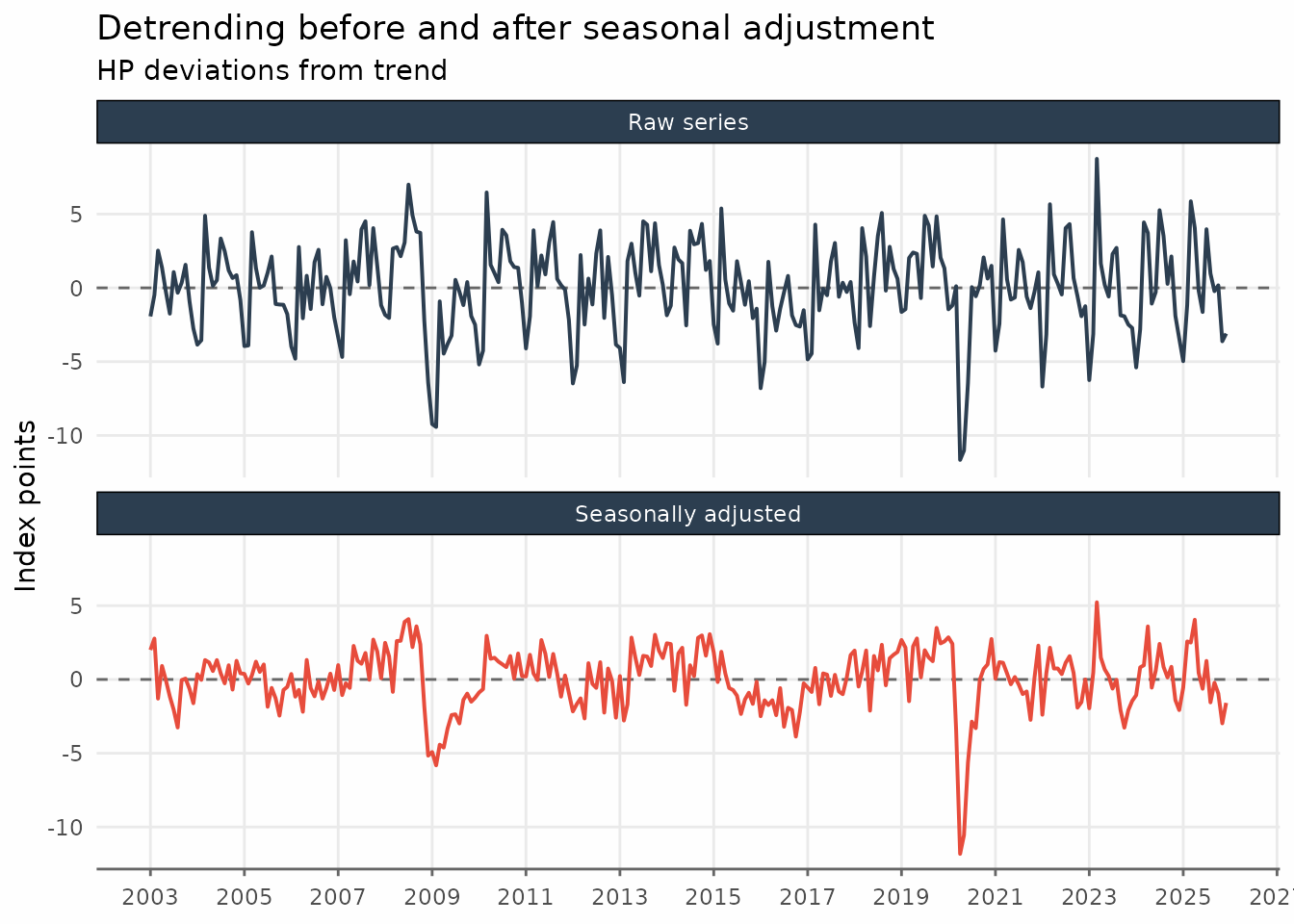
The seasonally adjusted cycle tells the same story more clearly. For seasonal data this two-step workflow — deseason, then detrend — should be the default.

Percentage deviations from trend

The ibcbr series is measured in index points, which makes it hard to compare across series or time periods. Macroeconomists usually report deviations as a percentage of the trend, the convention for output gaps.

Setting transform = "log" fits the trend on the log scale and returns the log deviation from trend, log(value) - log(trend). Multiplied by 100, this is approximately the percentage deviation. On the original scale the identity becomes multiplicative: value = trend * exp(detrend).

ibcbr_gap <- ibcbr |>
  deseason_series(value_col = "index") |>
  detrend_series(value_col = "seasadj_stl", transform = "log")

ggplot(ibcbr_gap, aes(date, detrend_hp)) +
  geom_hline(yintercept = 0, color = "gray40", lty = 2) +
  geom_line(lwd = 0.7) +
  scale_x_date(date_breaks = "2 years", date_labels = "%Y") +
  scale_y_continuous(labels = scales::percent) +
  labs(
    title = "An HP-filter activity gap",
    subtitle = "Log deviation from trend of the seasonally adjusted IBC-Br (x 100)",
    y = "% of trend"
  ) +
  theme_series

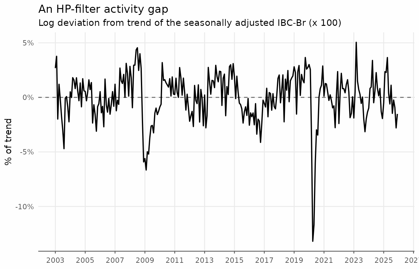
The COVID trough now reads directly as “activity was about 13% below trend”.

Comparing detrending methods

As with similar functions in trendseries, the methods argument accepts multiple methods in a single function call. Since the actual “cycle” is not observed, different filters take different stances on what counts as “trend”.

Passing several methods adds one detrend_* column per method, so the implied cycles can be compared side by side. Here we contrast the HP filter with the Hamilton filter, the regression-based alternative proposed by Hamilton (2018).

ibcbr_methods <- ibcbr |>
  deseason_series(value_col = "index") |>
  detrend_series(
    value_col = "seasadj_stl",
    methods = c("hp", "hamilton"),
    transform = "log"
  )

methods_long <- ibcbr_methods |>
  pivot_longer(
    cols = starts_with("detrend_"),
    names_to = "method",
    names_prefix = "detrend_",
    values_to = "cycle"
  )

ggplot(methods_long, aes(date, 100 * cycle)) +
  geom_hline(yintercept = 0, color = "gray40", lty = 2) +
  geom_line(aes(color = method), lwd = 0.7) +
  scale_x_date(date_breaks = "2 years", date_labels = "%Y") +
  labs(
    title = "HP vs Hamilton detrending",
    subtitle = "Log deviation from trend (x 100)",
    y = "% of trend",
    color = NULL
  ) +
  theme_series

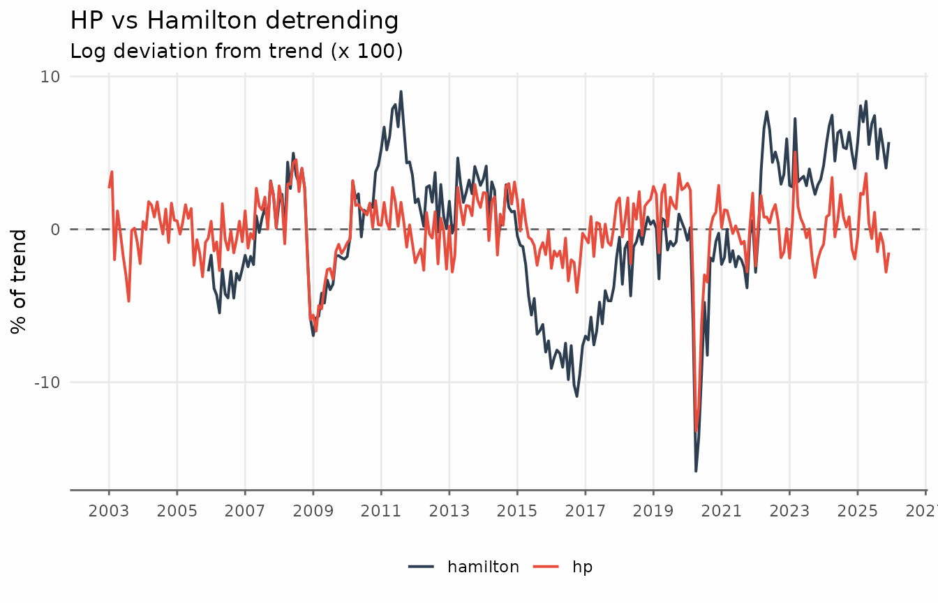
The two cycles agree on the major swings but differ in amplitude and timing — a useful reminder that detrended series are estimates, not data. Note also that the Hamilton filter projects the series two years ahead from a year of lags (h = 24, p = 12 for monthly data), so its first three years of detrended values are missing; methods with boundary effects (such as "bk") behave similarly at both ends.

The unified parameters of augment_trends() — window, smoothing, band, align, and params — all pass through unchanged. The Baxter-King filter, for instance, isolates fluctuations between 1.5 and 8 years directly.

ibcbr |>
  deseason_series(value_col = "index") |>
  detrend_series(
    value_col = "seasadj_stl",
    methods = "bk",
    band = c(18, 96) # periods in months
  )

The Econometric Filters vignette discusses what each of these filters does and how to choose between them.

Keeping the fitted trend

By default only the detrended column is added. Setting components = TRUE also keeps the fitted trend_* columns, which is handy for plotting the trend against the series or for verifying the identity.

ibcbr_parts <- ibcbr |>
  detrend_series(value_col = "index", components = TRUE)

all.equal(ibcbr_parts$trend_hp + ibcbr_parts$detrend_hp, ibcbr_parts$index)
#> [1] TRUE

ggplot(ibcbr_parts, aes(date)) +
  geom_line(aes(y = index, color = "Observed"), lwd = 0.7, alpha = 0.5) +
  geom_line(aes(y = trend_hp, color = "Trend (HP)"), lwd = 1) +
  scale_x_date(date_breaks = "2 years", date_labels = "%Y") +
  labs(
    title = "Economic activity and its HP trend",
    y = "Index (2003 = 100)",
    color = NULL
  ) +
  theme_series

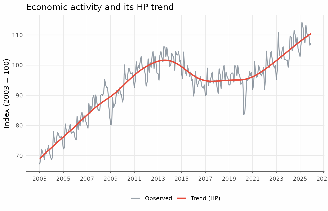
With transform = "log" the trend is reported back in the units of the series, so the same plot works unchanged.

Grouped detrending

Like the other functions in the package, detrend_series() accepts a group_cols argument to detrend several series at once. The full workflow — seasonal adjustment followed by detrending, in percent of trend — carries over group by group. Here we use the electricity dataset, which records monthly electricity consumption for three sectors.

elec_cycles <- electricity |>
  dplyr::filter(date >= as.Date("2003-01-01")) |>
  deseason_series(group_cols = "name_series") |>
  detrend_series(
    value_col = "seasadj_stl",
    group_cols = "name_series",
    transform = "log"
  )

glimpse(elec_cycles)
#> Rows: 828
#> Columns: 5
#> $ date        <date> 2003-01-01, 2003-02-01, 2003-03-01, 2003-04-01, 2003-05-0…
#> $ name_series <chr> "electric_commercial", "electric_commercial", "electric_co…
#> $ value       <dbl> 4182, 4153, 4221, 3948, 3938, 3711, 3667, 3720, 3686, 4001…
#> $ seasadj_stl <dbl> 3862.461, 3819.806, 3778.933, 3678.709, 4063.355, 4147.311…
#> $ detrend_hp  <dbl> 0.004224489, -0.011316838, -0.026511318, -0.057827607, 0.0…

ggplot(elec_cycles, aes(date, detrend_hp)) +
  geom_hline(yintercept = 0, color = "gray40", lty = 2) +
  geom_line(color = "#2c3e50", lwd = 0.7) +
  facet_wrap(vars(name_series), ncol = 1) +
  scale_x_date(date_breaks = "5 years", date_labels = "%Y") +
  scale_y_continuous(labels = scales::percent) +
  labs(
    title = "Electricity consumption cycles by sector",
    subtitle = "Log deviation from HP trend of the seasonally adjusted series (x 100)",
    y = "% of trend"
  ) +
  theme_series

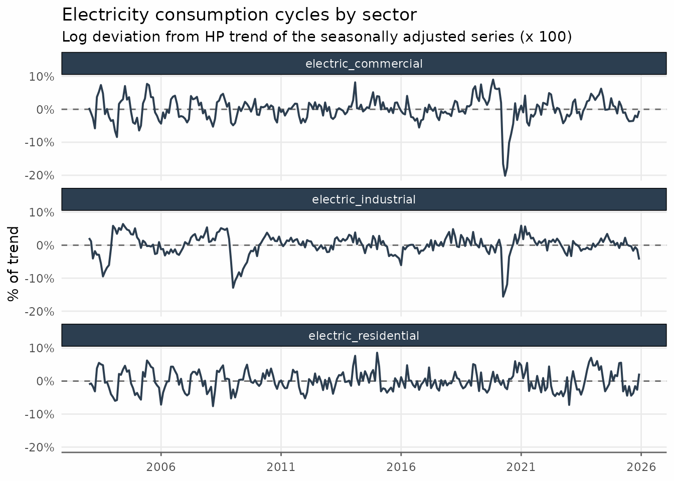
Commercial consumption swings the hardest — the collapse of in-person services during COVID stands out — while industrial demand stays closest to its trend.

Summary

detrend_series() removes the trend from a series, adding a detrend_{method} column with the deviation from trend (the cycle), so that value = trend + detrend.
Any trend method of augment_trends() can be used; the default is the HP filter with frequency-appropriate smoothing.
Detrending does not remove seasonality: for seasonal data, run deseason_series() first and detrend the seasadj_* column.
Use transform = "log" for deviations in percent of trend (the output-gap convention); the identity becomes value = trend * exp(detrend).
components = TRUE keeps the fitted trend columns alongside the detrended series.