Decomposing Series

The trend extraction methods covered in the other vignettes return a single smooth component. Often, though, an economic series is more naturally described as the sum of three parts: a slow-moving trend, a repeating seasonal pattern, and an irregular remainder. decompose_series() splits a series into these three components and adds them as columns to the original data frame.

library(trendseries)
library(dplyr)
library(tidyr)

The theme below is used throughout the vignette for consistent styling.

library(ggplot2)

theme_series <- theme_minimal(paper = "#fefefe") +
  theme(
    legend.position = "bottom",
    panel.grid.minor = element_blank(),
    strip.background = element_rect(fill = "#2c3e50"),
    strip.text = element_text(color = "#fefefe"),
    axis.ticks.x = element_line(color = "gray40", linewidth = 0.5),
    axis.line.x = element_line(color = "gray40", linewidth = 0.5),
    axis.title.x = element_blank(),
    palette.colour.discrete = c(
      "#2c3e50",
      "#e74c3c",
      "#f39c12",
      "#1abc9c",
      "#9b59b6"
    )
  )

Trend extraction vs decomposition

It is worth being clear about the difference between this function and augment_trends().

augment_trends() returns only the trend (trend_* columns). The seasonal and irregular movements are simply smoothed away.
decompose_series() returns all three components (trend_*, seasonal_*, and remainder_*), and they add back up exactly to the original series.

Because there is a seasonal component, decompose_series() requires seasonal data: monthly (frequency = 12) or quarterly (frequency = 4). For annual series there is nothing seasonal to isolate, so use augment_trends() instead.

A first decomposition

Let’s start with the gdp_construction dataset, a quarterly index of Brazilian construction activity that ships with trendseries.

ggplot(gdp_construction, aes(date, index)) +
  geom_line(lwd = 0.7) +
  scale_x_date(date_breaks = "2 years", date_labels = "%Y") +
  labs(
    title = "Brazilian construction activity",
    y = "Index"
  ) +
  theme_series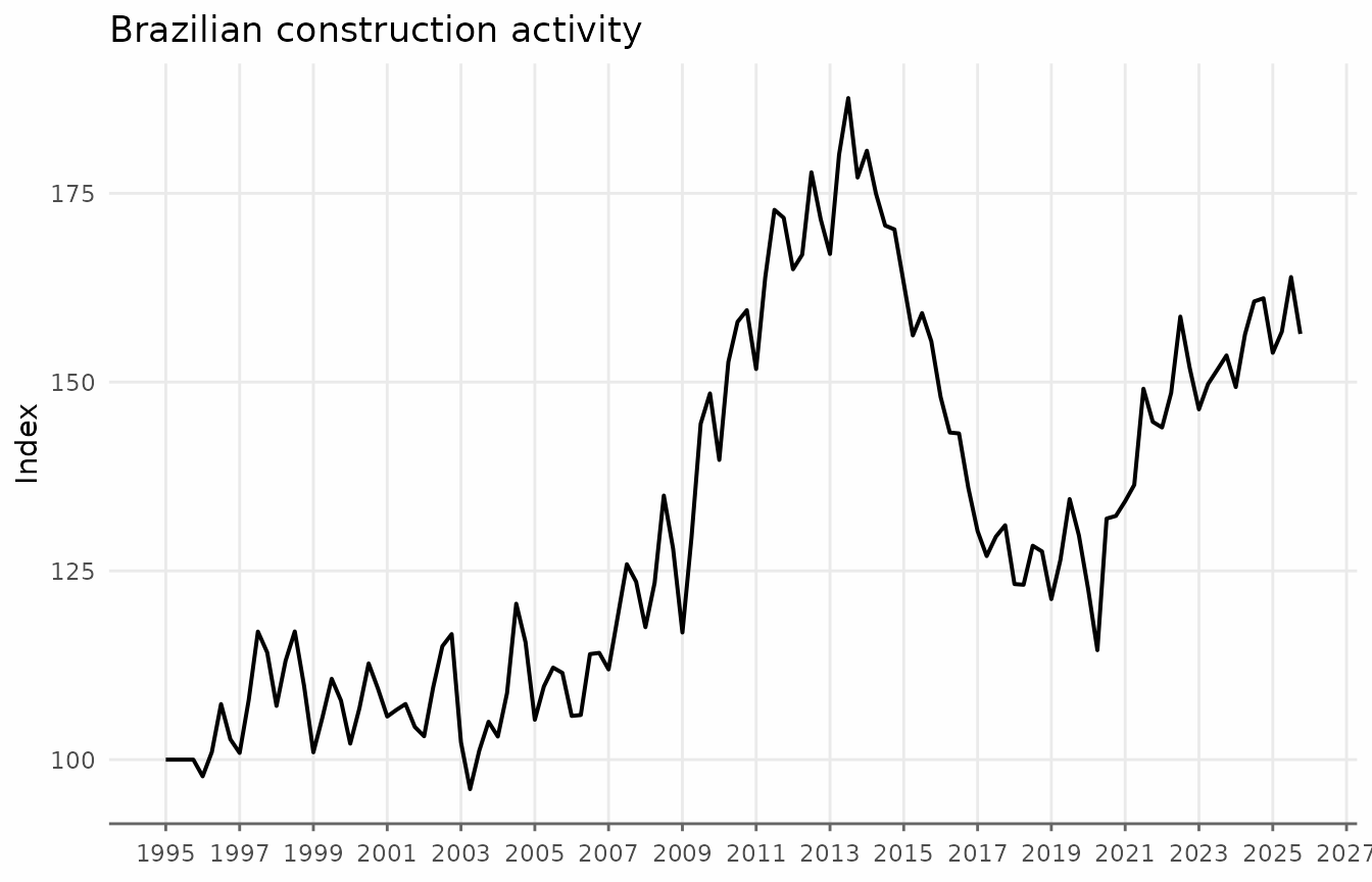

Passing the data to decompose_series() adds three new columns. The frequency is detected automatically from the date column.

gdp_parts <- gdp_construction |>
  decompose_series(value_col = "index")

gdp_parts
#> # A tibble: 124 × 5
#>    date       index trend_stl seasonal_stl remainder_stl
#>    <date>     <dbl>     <dbl>        <dbl>         <dbl>
#>  1 1995-01-01 100       102.         -4.37         1.93 
#>  2 1995-04-01 100       101.         -1.62         0.476
#>  3 1995-07-01 100       100.          4.44        -4.62 
#>  4 1995-10-01 100        99.4         1.55        -0.946
#>  5 1996-01-01  97.8     101.         -4.37         1.42 
#>  6 1996-04-01 101.      102.         -1.62         0.613
#>  7 1996-07-01 107.      103.          4.44         0.370
#>  8 1996-10-01 103.      104.          1.55        -2.49 
#>  9 1997-01-01 101.      106.         -4.37        -0.530
#> 10 1997-04-01 108.      109.         -1.62         0.849
#> # ℹ 114 more rows

The three components are named after the method (stl by default): trend_stl, seasonal_stl, and remainder_stl.

Reshaping to long format makes it easy to plot the original series alongside its three components.

gdp_long <- gdp_parts |>
  pivot_longer(
    cols = c(index, trend_stl, seasonal_stl, remainder_stl),
    names_to = "component",
    values_to = "value"
  ) |>
  mutate(
    component = factor(
      component,
      levels = c("index", "trend_stl", "seasonal_stl", "remainder_stl"),
      labels = c("Observed", "Trend", "Seasonal", "Remainder")
    )
  )

ggplot(gdp_long, aes(date, value)) +
  geom_line(aes(color = component), lwd = 0.7, show.legend = FALSE) +
  facet_wrap(vars(component), ncol = 1, scales = "free_y") +
  scale_x_date(date_breaks = "2 years", date_labels = "%Y") +
  labs(
    title = "STL decomposition of construction activity",
    subtitle = "Observed = Trend + Seasonal + Remainder",
    y = NULL
  ) +
  theme_series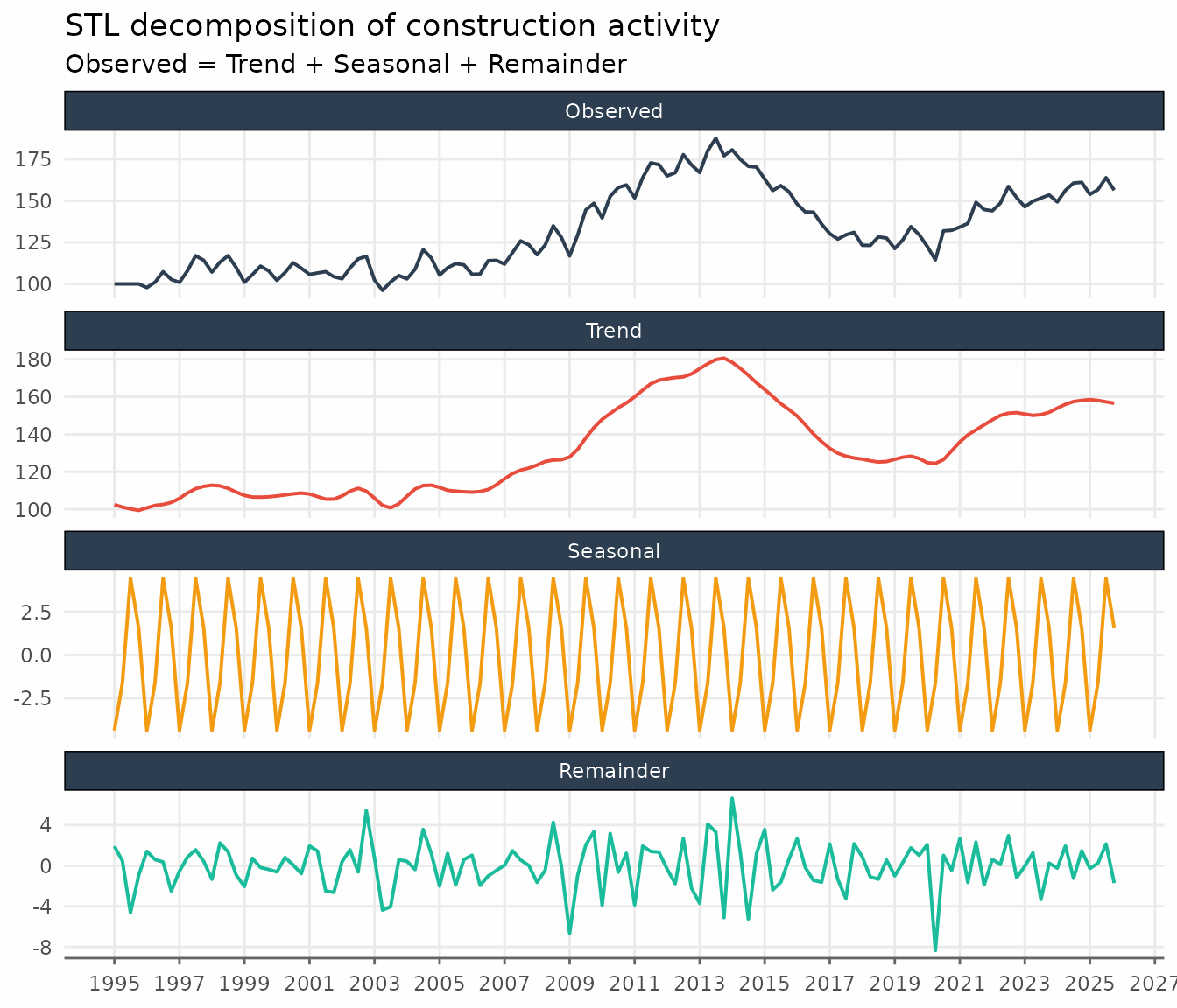

STL decomposition

The default method is STL (Seasonal-Trend decomposition via Loess), implemented with stats::stl(). The seasonal component is estimated with a loess smoother, the trend with an adaptive moving average, and the remainder is whatever is left over. The defaults (s.window = "periodic", robust = FALSE) suit most economic series with a stable seasonal pattern.

Fine control is available through the params list. The two most useful options are an evolving seasonal pattern and robust fitting.

# Allow the seasonal pattern to evolve slowly over time, and downweight outliers
gdp_robust <- gdp_construction |>
  decompose_series(
    value_col = "index",
    params = list(s.window = 13, robust = TRUE)
  )

A s.window of "periodic" forces an identical seasonal shape in every year; supplying a positive odd integer instead lets that shape drift gradually. Setting robust = TRUE reduces the influence of one-off spikes on the trend and seasonal estimates.

Regression decomposition

The regression method (methods = "regression") fits a single OLS model

$y_t = f(t) + s(t) + \epsilon_t$

where $f(t)$ is a polynomial in time and $s(t)$ is a set of period (month or quarter) dummy variables. The trend is the constant plus the polynomial terms, the seasonal component is the period effect (centred to mean zero), and the remainder is the model residual.

Unlike STL, the regression trend is a smooth global polynomial, which can be a better description of a series with a steady long-run direction. For the examples that follow we use the oil_derivatives dataset, which records monthly petroleum-derivatives production in Brazil; we restrict it to the 1995–2006 window and work on the log scale.

suboil <- oil_derivatives |>
  filter(between(date, as.Date("1995-06-01"), as.Date("2006-12-01"))) |>
  mutate(lprod = log(production))

ggplot(suboil, aes(date, lprod)) +
  geom_line(lwd = 0.7) +
  labs(
    title = "Petroleum derivatives production",
    y = "Thousand barrels per day (log scale)"
  ) +
  theme_series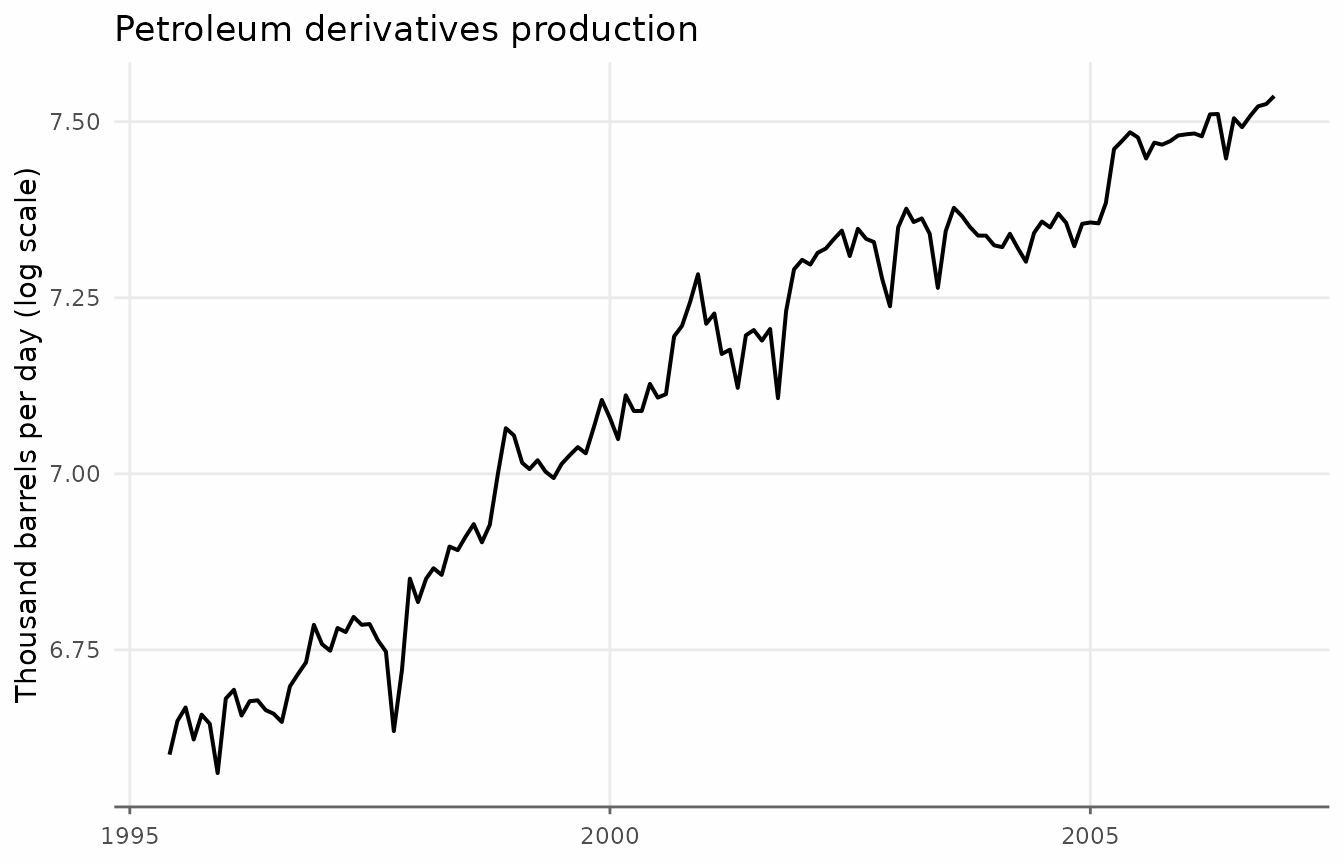

The trend argument selects the polynomial form: "linear" (the default), "quadratic", or "cubic". Orthogonal polynomials are used by default for numerical stability.

suboil_reg <- suboil |>
  decompose_series(
    value_col = "lprod",
    methods = "regression",
    trend = "cubic"
  )

ggplot(suboil_reg, aes(date)) +
  geom_line(aes(y = lprod, color = "Original"), lwd = 0.7) +
  geom_line(aes(y = trend_regression, color = "Trend (reg.)"), lwd = 0.7) +
  labs(title = "Regression cubic trend", y = "log production", color = NULL) +
  theme_series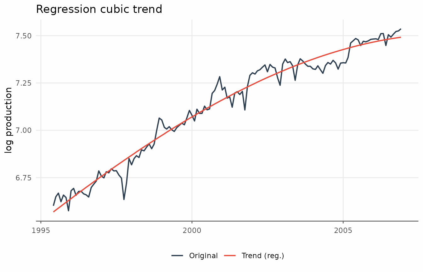

If the series is trend-stationary, remainder_regression — the series with the trend and seasonality removed — is approximately stationary.

ggplot(suboil_reg, aes(date, remainder_regression)) +
  geom_line(lwd = 0.7) +
  labs(title = "Regression remainder", y = NULL) +
  theme_series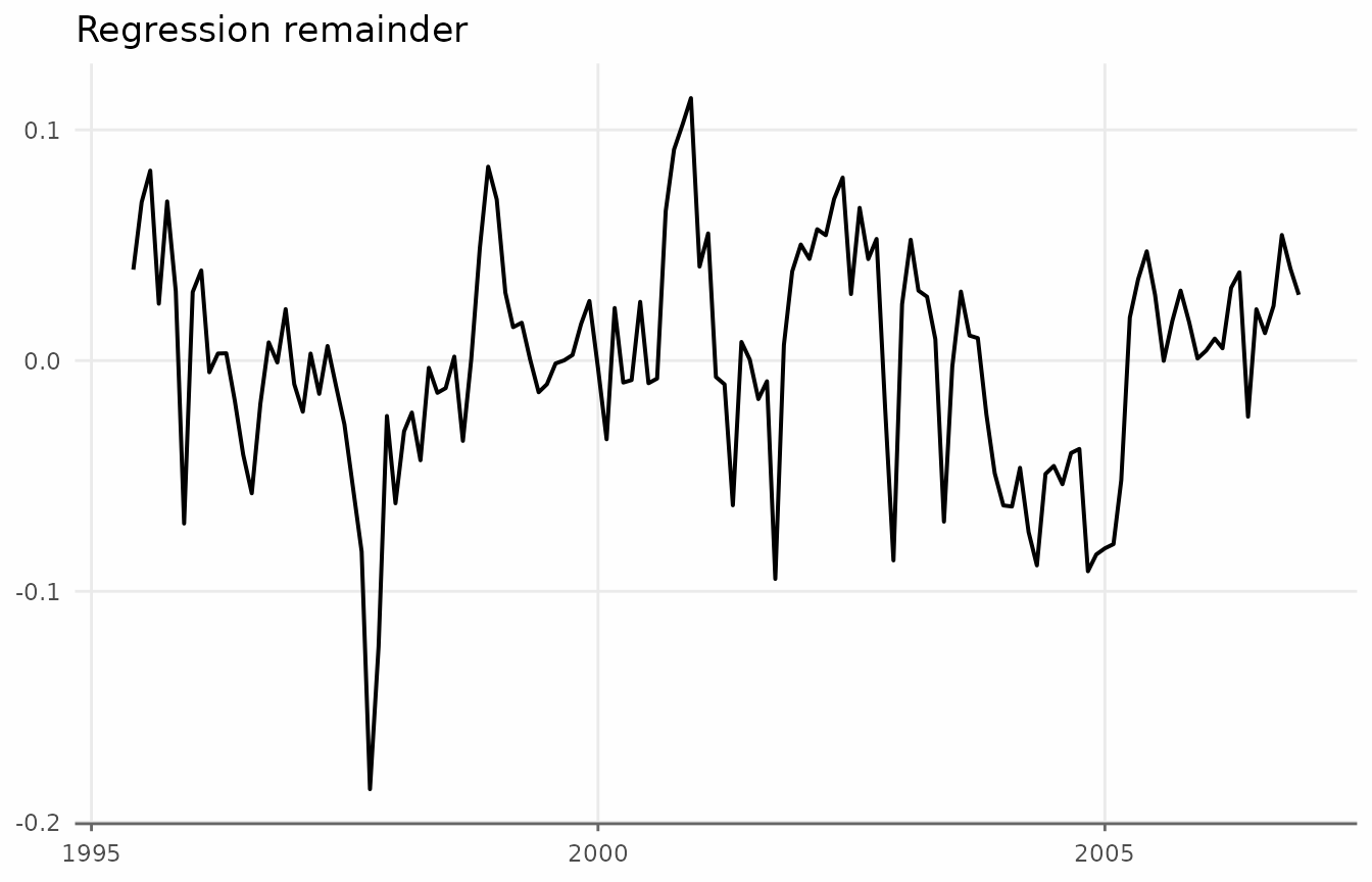

It is instructive to compare the two decomposition methods directly. Both produce fixed seasonal patterns, but STL follows short-term fluctuations more closely, producing a “cleaner” remainder.

comparison <- suboil |>
  decompose_series(value_col = "lprod", methods = "stl") |>
  decompose_series(value_col = "lprod", methods = "regression", trend = "cubic")

comparison_long <- comparison |>
  pivot_longer(
    cols = trend_stl:remainder_regression,
    names_pattern = "(.*)_(.*)",
    names_to = c("component", "method"),
    values_to = "trend"
  ) |>
  mutate(
    component = factor(component, levels = c("trend", "seasonal", "remainder"))
  )

ggplot(comparison_long, aes(date, trend)) +
  # Original series
  geom_line(
    data = suboil,
    aes(y = lprod),
    layout = c(1, 2),
    lwd = 0.5,
    alpha = 0.5
  ) +
  # Components and methods
  geom_line(aes(y = trend, color = component), lwd = 0.7) +
  facet_grid(vars(component), vars(method), scales = "free_y") +
  guides(color = "none") +
  labs(title = "STL vs regression decomposition", y = NULL) +
  theme_series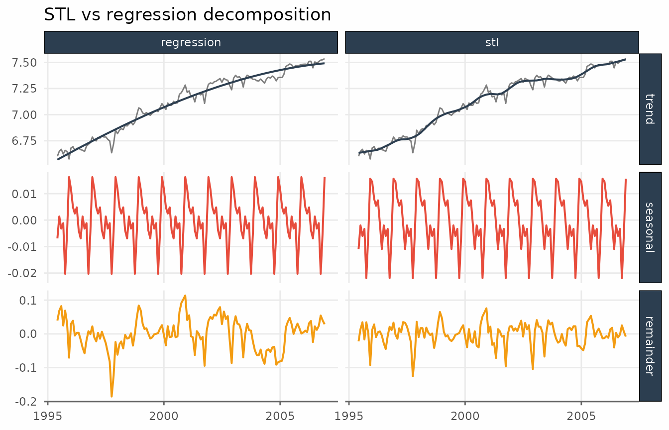

Grouped decomposition

Like augment_trends(), decompose_series() accepts a group_cols argument to decompose several series at once. The data must be in tidy long format. Here we use the electricity dataset, which records monthly electricity consumption for three sectors (residential, commercial, and industrial).

electricity_parts <- electricity |>
  mutate(lvalue = log(value)) |>
  decompose_series(value_col = "lvalue", group_cols = "name_series")

glimpse(electricity_parts)
#> Rows: 1,689
#> Columns: 7
#> $ date          <date> 1979-02-01, 1979-03-01, 1979-04-01, 1979-05-01, 1979-06…
#> $ name_series   <chr> "electric_commercial", "electric_commercial", "electric_…
#> $ value         <dbl> 1030, 1057, 1044, 1038, 1002, 979, 985, 1047, 1067, 1113…
#> $ lvalue        <dbl> 6.937314, 6.963190, 6.950815, 6.945051, 6.909753, 6.8865…
#> $ trend_stl     <dbl> 6.908726, 6.918239, 6.927753, 6.937020, 6.946288, 6.9554…
#> $ seasonal_stl  <dbl> 0.04401996, 0.04635439, 0.04502582, -0.01022254, -0.0527…
#> $ remainder_stl <dbl> -0.015431723, -0.001403624, -0.021963659, 0.018253335, 0…

Each group is decomposed independently, and the components are stacked back into a single data frame.

ggplot(electricity_parts, aes(date)) +
  geom_line(aes(y = seasonal_stl), color = "#2c3e50", lwd = 0.8) +
  facet_wrap(vars(name_series), ncol = 1, scales = "free_y") +
  scale_x_date(date_breaks = "3 years", date_labels = "%Y") +
  labs(
    title = "Electricity consumption by sector",
    subtitle = "STL seasonal component extracted per group (log scale)",
    y = "seasonal factor (log)"
  ) +
  theme_series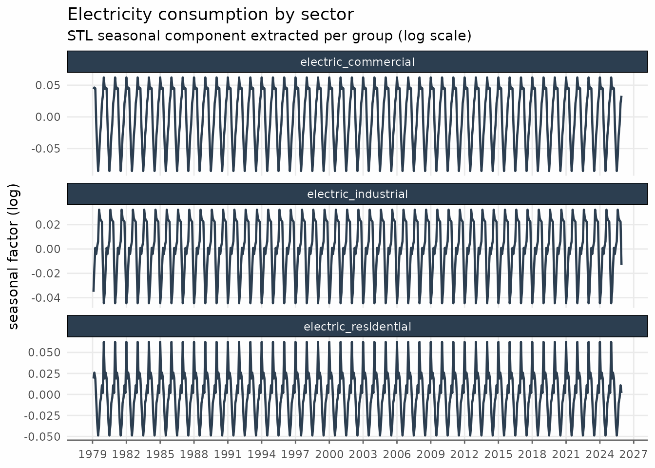

Multiplicative seasonality

So far we have handled multiplicative seasonality by logging the series before decomposing (lprod = log(production), lvalue = log(value)). Many macroeconomic series behave this way: the seasonal variations grow with the level of the series, so an additive decomposition of the raw data would leave a seasonal pattern that widens over time.

Every decompose_series() method is additive by construction. Instead of logging manually, you can pass transform = "log", which logs the series, decomposes it additively, and exponentiates the components back to the original scale.

decompose_series(
  oil_derivatives,
  value_col = "production",
  transform = "log"
)

On the log scale the additive identity holds; after exponentiating, the components satisfy the multiplicative identity trend * seasonal * remainder = value. This requires strictly positive data.

Other methods

Classical decomposition

methods = "classic" is the textbook decomposition implemented by stats::decompose(). The trend is a centred moving average of order equal to the frequency, the seasonal component is the average detrended value for each period, and the remainder is what is left. It is simple and fast, but shouldn’t be used in practice.

decompose_series(
  oil_derivatives,
  value_col = "production",
  methods = "classic",
  transform = "log"
)

Basic structural model

methods = "bsm" fits a Basic Structural (state-space) Model with stats::StructTS(): stochastic level, slope, and seasonal components estimated by maximum likelihood and extracted with the Kalman smoother. Unlike the moving-average methods, it returns trend and seasonal estimates for every observation and lets both components evolve over time. The trade-off is that it relies on numerical optimisation, which can occasionally fail to converge on short or irregular series.

decompose_series(
  suboil,
  value_col = "lprod",
  methods = "bsm"
)

X-13ARIMA-SEATS (`seasonal`)

methods = "seats" runs the U.S. Census Bureau’s X-13ARIMA-SEATS program through the seasonal package — the seasonal-adjustment procedure used by many statistical agencies. seas() is called with its automatic defaults: ARIMA model selection, log/level transformation, outlier detection, and calendar adjustment. The SEATS trend-cycle and seasonally adjusted series are then mapped to a trend/seasonal/remainder triple that reproduces the original series exactly. Because X-13 selects its own transformation internally, there is normally no need to set transform = "log" for this method.

# requires the 'seasonal' package
seas_oil <- decompose_series(
  suboil,
  value_col = "lprod",
  methods = "seats"
)

ggplot(seas_oil, aes(date)) +
  geom_line(aes(y = lprod, color = "Original"), lwd = 0.7) +
  geom_line(aes(y = trend_seats, color = "Trend (SEATS)"), lwd = 0.7) +
  labs(title = "SEATS trend-cycle", y = "log production") +
  theme_series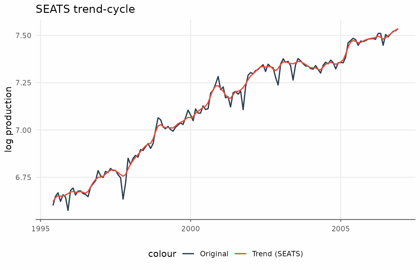

ggplot(seas_oil, aes(date, seasonal_seats)) +
  geom_line(lwd = 0.7) +
  labs(title = "SEATS seasonal component", y = NULL) +
  theme_series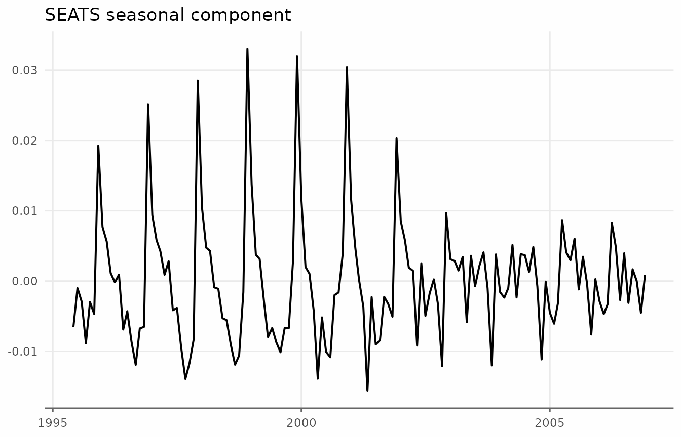

Often our interest is mainly in the series without its seasonal component. For convenience, deseason_series() wraps decompose_series() and returns the seasonally adjusted series directly.

deseas_oil <- deseason_series(
  suboil,
  value_col = "lprod",
  methods = "seats",
  # set to TRUE to also return the trend, seasonal, and remainder components
  components = FALSE
)

ggplot(deseas_oil, aes(date, seasadj_seats)) +
  geom_line(lwd = 0.7) +
  labs(
    title = "SEATS seasonally adjusted series",
    y = "log production"
  ) +
  theme_series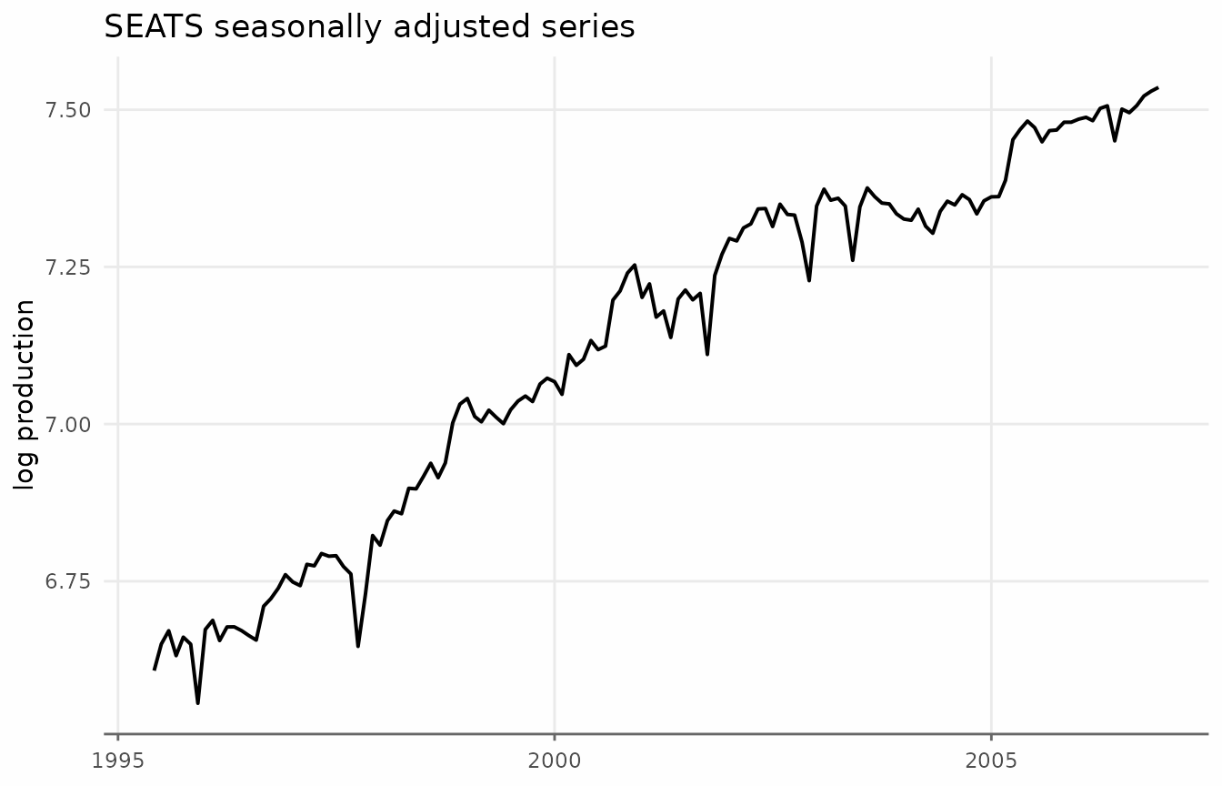

This is equivalent to using seasadj = TRUE in decompose_series().

decompose_series(
  suboil,
  value_col = "lprod",
  methods = "seats",
  seasadj = TRUE
)

Summary

decompose_series() splits a seasonal (monthly or quarterly) series into trend, seasonal, and remainder components that sum to the original series.
There are five available methods: "stl" (default), "regression", "classic", "bsm", and "seats"
All methods are additive; use transform = "log" for multiplicative seasonality, where the components instead multiply to the original series.
deseason_series() is a convenience wrapper that returns only the seasonally adjusted series.

Decomposing Series