The Primary Market and the Construction Cycle • realestatebr

This article follows the development cycle, from launches to sales and deliveries, and the business environment around it. Three datasets do the work.

abrainc for national primary market indicators from the ABRAINC-FIPE panel of developers
secovi for the São Paulo market
fgv_ibre for construction costs and business sentiment

The aim is to show what these datasets hold, not to settle any question about the market. Besides the usual dplyr and ggplot2, we use the trendseries package to estimate trends and cycles.

library(realestatebr)
library(trendseries)
library(dplyr)
library(ggplot2)

The code below defines a common theme for the plots in this article and can be omitted.

library(ekioplot)
color_palette <- ekioplot::ekio_pal()
theme_series <- function() {
  ekioplot::theme_ekio(base_size = 10) +
    theme(
      palette.color.discrete = color_palette
    )
}

Construction costs and sentiment

The fgv_ibre dataset gathers indicators from Fundação Getulio Vargas (FGV). FGV runs a wide range of surveys, and realestatebr collects the ones most relevant to construction and real estate. The name_series and code_series columns identify each series.

fgv <- get_dataset("fgv_ibre")

count(fgv, name_series, name_simplified)
#> # A tibble: 15 × 3
#>    name_series                                             name_simplified     n
#>    <chr>                                                   <chr>           <int>
#>  1 ICST Com ajuste Sazonal - Índice de Confiança da Const… ic_cst            193
#>  2 IE-CST Com ajuste Sazonal - Índice de Expectativas da … ie_cst            193
#>  3 INCC - 1o Decendio                                      incc_1o_decend…   259
#>  4 INCC - 2o Decendio                                      incc_2o_decend…   259
#>  5 INCC - Brasil                                           incc_brasil       361
#>  6 INCC - Brasil - DI                                      incc_brasil_di    360
#>  7 INCC - Brasil-10                                        incc_brasil_10    361
#>  8 INCC - Fechamento Mensal                                incc              361
#>  9 ISA-CST Com ajuste Sazonal - Índice da Situação Atual … isa_cst           193
#> 10 Sondagem da Construção – Nível de Utilização da Capaci… nuci              160
#> 11 Índice de Variação de Aluguéis Residenciais (IVAR) - B… ivar_belo_hori…    91
#> 12 Índice de Variação de Aluguéis Residenciais (IVAR) - M… ivar_brazil        91
#> 13 Índice de Variação de Aluguéis Residenciais (IVAR) - P… ivar_porto_ale…    91
#> 14 Índice de Variação de Aluguéis Residenciais (IVAR) - R… ivar_rio_de_ja…    91
#> 15 Índice de Variação de Aluguéis Residenciais (IVAR) - S… ivar_sao_paulo     91

The plot below shows the confidence indicators of the construction sector. ICST is the overall index, which averages the IE-CST (expectations) and the ISA-CST (current situation). Although these series are already seasonally adjusted, we smooth them with a 12-month moving average to make them more stable. As with most confidence indicators, the values are normalized: values above 100 indicate a more favorable assessment, while values below 100 indicate a less favorable assessment.

confidence <- fgv |>
  filter(name_simplified %in% c("ic_cst", "ie_cst", "isa_cst")) |>
  augment_trends(group_cols = "name_simplified", methods = "ma") |>
  mutate(
    indicator = case_when(
      name_simplified == "ic_cst" ~ "ICST",
      name_simplified == "ie_cst" ~ "IE-CST (Expectations)",
      name_simplified == "isa_cst" ~ "ISA-CST (Current Situation)"
    )
  )

ggplot(confidence, aes(date, trend_ma)) +
  geom_line(aes(color = indicator), lwd = 0.8) +
  geom_hline(yintercept = 100) +
  labs(
    title = "Confidence Indicators",
    subtitle = "Construction sector confidence indicators, 12-month moving average.",
    y = "Index",
    color = NULL
  ) +
  theme_series()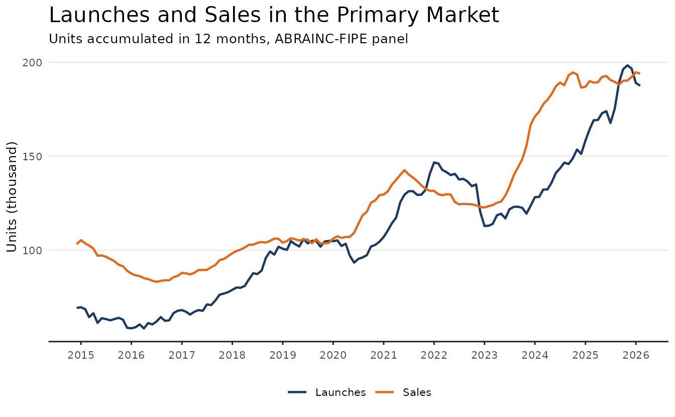

Launches and sales

The indicator table from abrainc reports monthly launches, sales, deliveries, cancellations, and supply for a panel of large developers. The series are volatile, so the plot below uses values accumulated over twelve months.

abrainc <- get_dataset("abrainc", table = "indicator")

glimpse(abrainc)
#> Rows: 3,552
#> Columns: 6
#> $ date           <date> 2014-01-01, 2014-01-01, 2014-01-01, 2014-01-01, 2014-0…
#> $ year           <dbl> 2014, 2014, 2014, 2014, 2014, 2014, 2014, 2014, 2014, 2…
#> $ category       <chr> "new_units", "new_units", "new_units", "new_units", "so…
#> $ variable       <chr> "total", "market_rate", "social_housing", "other", "tot…
#> $ value          <dbl> 1726.0000, NA, NA, NA, 4232.0000, NA, NA, NA, 6409.0000…
#> $ variable_label <chr> "Total", "Market-rate Development", "Social Housing (MC…

abrainc_trends <- abrainc |>
  filter(
    category %in% c("new_units", "sold"),
    variable == "total"
  ) |>
  mutate(
    units_12m = zoo::rollsumr(value, k = 12, fill = NA) / 1e3,
    category_label = case_when(
      category == "new_units" ~ "Launches",
      category == "sold" ~ "Sales",
      TRUE ~ NA_character_
    )
  ) |>
  trendseries::augment_trends(
    value_col = "units_12m",
    group_cols = "category_label"
  )

ggplot(abrainc_trends, aes(date, units_12m, color = category_label)) +
  geom_line(lwd = 0.5, alpha = 0.5) +
  geom_line(aes(y = trend_stl), lwd = 0.8) +
  facet_wrap(vars(category_label), ncol = 1) +
  scale_x_date(date_breaks = "1 year", date_labels = "%Y") +
  labs(
    title = "Launches and Sales in the Primary Market",
    subtitle = "Units accumulated in 12 months, ABRAINC-FIPE panel",
    y = "Units (thousand)",
    color = NULL
  ) +
  theme_series()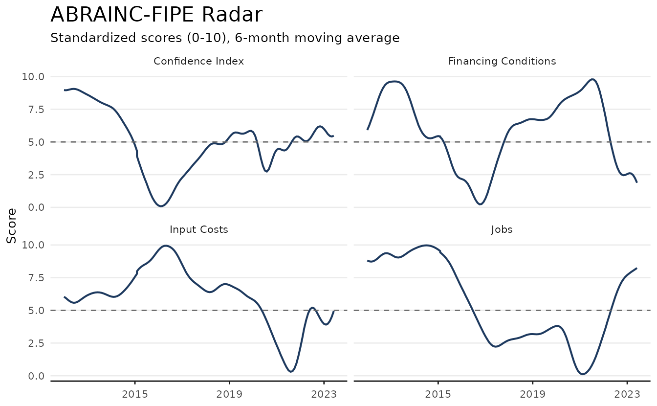

Market segments

Brazil has two large segments: (1) social housing production, which is financed and subsidized by the “Minha Casa Minha Vida” program (usually abbreviated as “MCMV”); and (2) market-rate developments. The ABRAINC dataset reports sales and launches for each of these markets.

segments <- abrainc |>
  filter(
    category == "sold",
    variable %in% c("market_rate", "social_housing")
  ) |>
  summarise(
    year_total = if (anyNA(value)) NA_real_ else sum(value) / 1e3,
    .by = c("variable_label", "year")
  ) |>
  filter(!is.na(year_total))

ggplot(segments, aes(year, year_total)) +
  geom_col(aes(fill = variable_label)) +
  scale_x_continuous(breaks = scales::breaks_pretty(n = 8)) +
  scale_y_continuous(expand = expansion(mult = c(0, 0.05))) +
  labs(
    title = "Sales by Market Segment",
    subtitle = "Total yearly sales by market segment.",
    y = "Units (thousand)",
    fill = NULL
  ) +
  theme_series()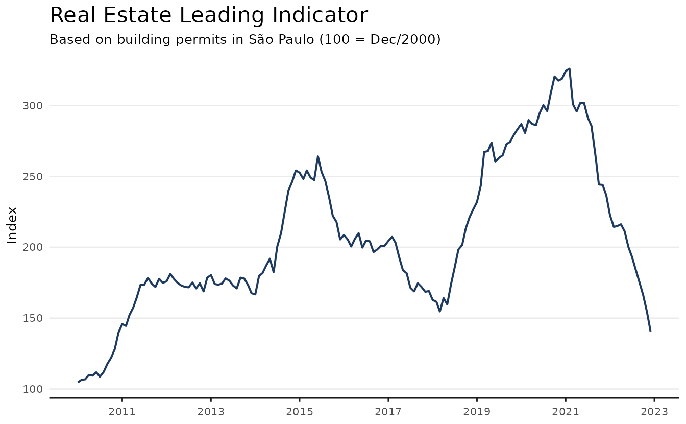

Business conditions

The radar table condenses the business environment into standardized 0-10 scores across four dimensions: (1) macroeconomy; (2) credit; (3) demand; and (4) the real estate sector. The plot shows one representative indicator from each dimension, smoothed with a six-month moving average. Note that the moving average is already bundled with the data in the ma6 column.

radar <- get_dataset("abrainc", table = "radar")

radar_sel <- radar |>
  filter(
    variable %in%
      c("confidence", "finance_condition", "employment", "input_costs"),
    date >= as.Date("2012-01-01")
  )

ggplot(radar_sel, aes(date, ma6)) +
  geom_line(color = color_palette[1], lwd = 0.8) +
  geom_hline(yintercept = 5, linetype = 2, color = "gray40") +
  facet_wrap(vars(variable_label)) +
  scale_x_date(date_breaks = "4 years", date_labels = "%Y") +
  labs(
    title = "ABRAINC-FIPE Radar",
    subtitle = "Standardized scores (0-10), 6-month moving average.",
    y = "Score"
  ) +
  theme_series()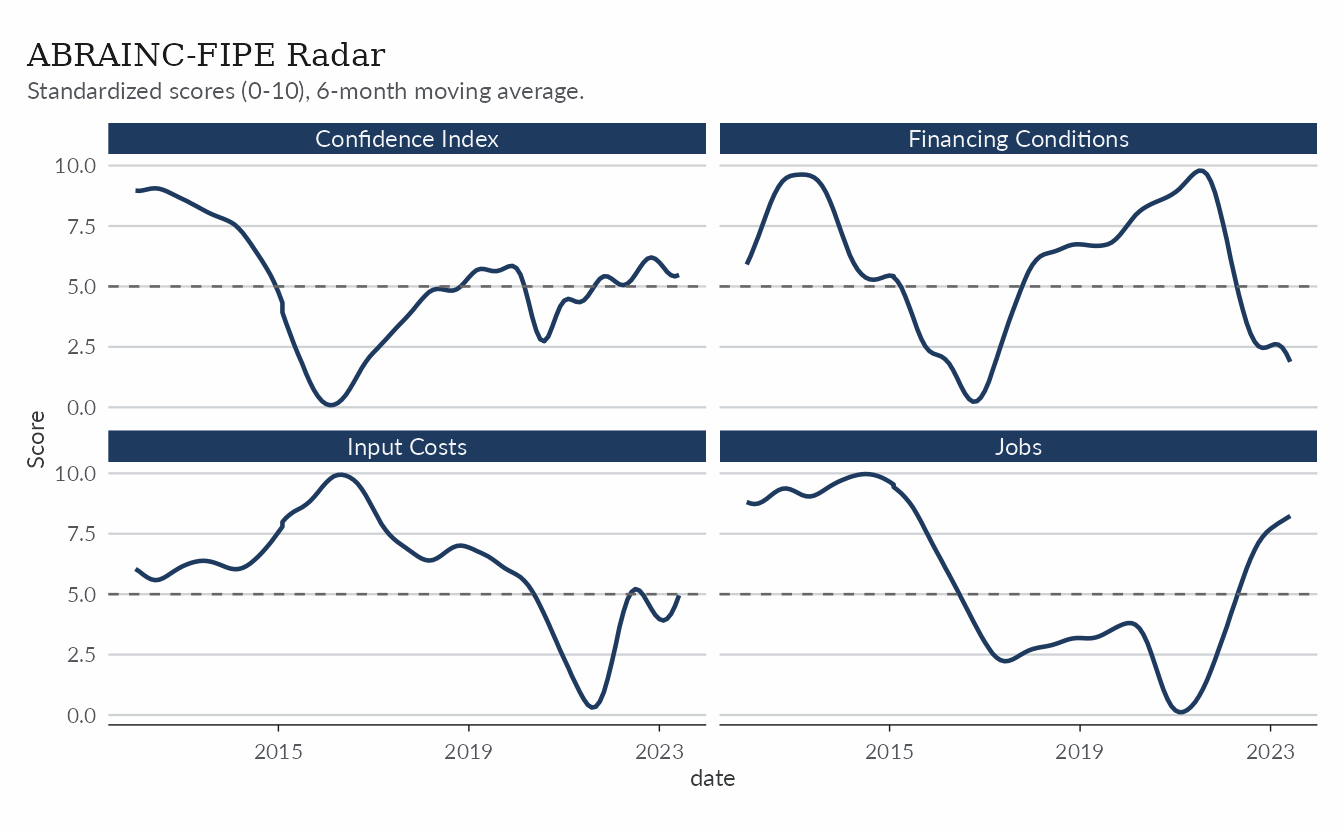

The radar indicator has been discontinued upstream, so the series ends at its last published month. The GitHub issue tracks its status.

São Paulo

São Paulo is Brazil’s largest real estate market, and two sources cover it here. The leading table from abrainc reports building permits in the city, while secovi reports supply and sales for the city and the metropolitan region.

A leading indicator

Building permits anticipate construction activity. The leading table compiles permits in the city of São Paulo into a leading indicator of real estate activity.

leading <- get_dataset("abrainc", table = "leading")

leading_index <- leading |>
  filter(
    variable == "leading_index",
    zone != "Total",
    date >= as.Date("2010-01-01")
  )

ggplot(leading_index, aes(date, value)) +
  geom_line(color = color_palette[1], lwd = 0.8) +
  facet_wrap(vars(zone)) +
  scale_x_date(date_breaks = "2 years", date_labels = "%Y") +
  labs(
    title = "Real Estate Leading Indicator",
    subtitle = "Based on building permits in São Paulo (100 = Dec/2000)",
    y = "Index"
  ) +
  theme_series()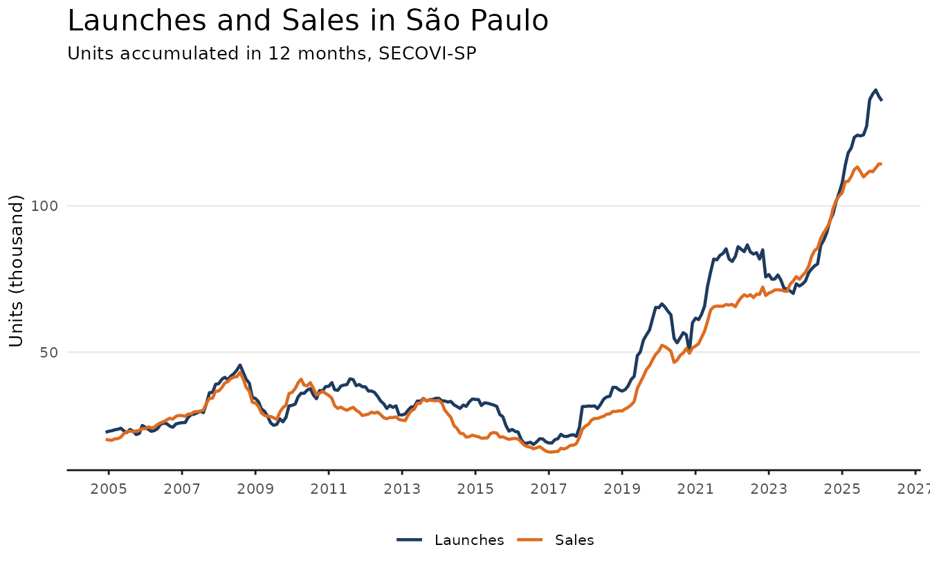

Supply and sales

The launch and sale tables from secovi track new supply and sales in the city.

secovi <- get_dataset("secovi")

count(secovi, category, variable)
#> # A tibble: 12 × 3
#>    category variable               n
#>    <chr>    <chr>              <int>
#>  1 condo    default_condominio   240
#>  2 condo    icon                1746
#>  3 launch   launches             538
#>  4 launch   supply               269
#>  5 rent     acao_locaticia      1980
#>  6 rent     rent_price           236
#>  7 rent     tipos_de_garantia    618
#>  8 sale     sales                807
#>  9 sale     sales_1rooms         807
#> 10 sale     sales_2rooms         807
#> 11 sale     sales_3rooms         807
#> 12 sale     sales_4rooms         807

sp_market <- secovi |>
  filter(
    variable %in% c("launches", "sales"),
    name == "unidades"
  ) |>
  mutate(
    units_12m = zoo::rollsumr(value, k = 12, fill = NA) / 1e3
  ) |>
  trendseries::augment_trends(
    value_col = "units_12m",
    group_cols = "variable"
  ) |>
  mutate(
    variable_label = if_else(variable == "launches", "Launches", "Sales")
  )

ggplot(sp_market, aes(date)) +
  geom_line(
    aes(y = units_12m, color = variable_label),
    lwd = 0.6,
    alpha = 0.5
  ) +
  geom_line(aes(y = trend_stl, color = variable_label), lwd = 0.8) +
  facet_wrap(vars(variable_label), ncol = 1) +
  scale_x_date(date_breaks = "2 years", date_labels = "%Y") +
  guides(color = "none") +
  labs(
    title = "Launches and Sales in São Paulo",
    subtitle = "Units accumulated in 12 months, SECOVI-SP",
    y = "Units (thousand)",
    color = NULL
  ) +
  theme_series()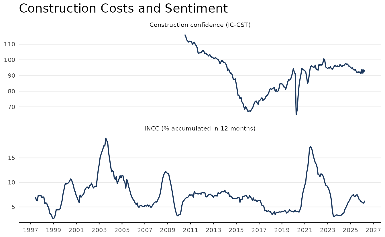

Some series break the totals down further. The plot below shows sales by number of rooms.

sp_market_rooms <- secovi |>
  filter(
    grepl("sales_[0-9]rooms", variable),
    name == "unidades"
  ) |>
  trendseries::augment_trends(group_cols = "variable") |>
  mutate(
    variable_label = regmatches(variable, regexpr("\\d+", variable)),
    variable_label = if_else(
      variable == "sales_1rooms",
      paste(variable_label, "room"),
      paste(variable_label, "rooms")
    )
  )

ggplot(sp_market_rooms, aes(date)) +
  geom_line(aes(y = trend_stl, color = variable_label), lwd = 0.8) +
  facet_wrap(vars(variable_label)) +
  scale_x_date(date_breaks = "2 years", date_labels = "%Y") +
  guides(color = "none") +
  labs(
    title = "Sales in São Paulo",
    subtitle = "STL trends for sales by number of rooms.",
    y = "Units (thousand)"
  ) +
  theme_series()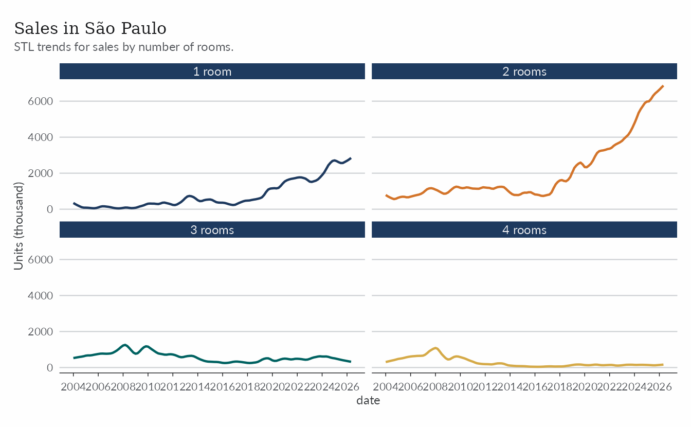

Learn more

The help topics ?abrainc, ?secovi, and ?fgv_ibre document the columns of each dataset used here. For housing credit, see Housing Credit in Brazil; for price indices, see Working with Property Price Indices.