Working with Property Price Indices

Introduction

This vignette provides a brief introduction to Residential Property Price Indices (RPPI) in the realestatebr package. Since realestatebr returns tibble as default values, we recommend using it together with the dplyr package, though conversion do data.table is trivial.

library(realestatebr)
library(dplyr)

The code below defines a common theme for all plots in this vignette and is required to fully replicate the code in this document. Despite this, this code is entirely optional and can be omitted.

library(ggplot2)

color_palette <- c(
  "#1E3A5F",
  "#DD6B20",
  "#2C7A7B",
  "#D69E2E",
  "#805AD5",
  "#C53030"
)

theme_series <- function() {
  theme_minimal(
    # swap for other font if needed
    base_family = "Avenir",
    base_size = 10
  ) +
    theme(
      plot.title = element_text(size = 16),
      panel.grid.minor = element_blank(),
      panel.grid.major.x = element_blank(),
      axis.line.x = element_line(color = "gray10", linewidth = 0.5),
      axis.ticks.x = element_line(color = "gray10", linewidth = 0.5),
      axis.title.x = element_blank(),
      legend.position = "bottom",
      palette.color.discrete = color_palette
    )
}

Brazil has several residential property price indices (RPPIs) from different institutions, each with distinct methodologies, geographic coverage, and time spans. This vignette shows how to access and work with each one.

Recommended Workflow

Before getting into all the details, it’s convenient to establish which are the “best” indices to use.

The best indices

The two most consistent indices are the IGMI-R (for sale prices) and the IVAR (for rent prices). The only available option for commercial prices is FipeZap. These indices are sourced from good datasets and are built with a robust methodology.

The IGMI-R is a hedonic price index based on transaction prices of housing mortgages. The only shortcoming of the index is its relatively short time span (2014-present) and geographic coverage (major cities only).

The IVAR is a repeat-rent index based on residential rental contracts. Unfortunately, the dataset has a very short time span (2019-present) and even more limited geographic coverage (only 4 cities).

FipeZap has the broadest geographic (50+ cities) and temporal coverage (2008-present), but is based on median listing prices rather than transaction prices. As a result, the index is much less reliable.

The IGMI-R and IVAR are the most precise indices for sales and rent, respectively, and should be used for most applications.

Working with realestatebr

To get a dataset, use get_dataset()

igmi <- get_dataset("rppi", table = "igmi")
ivar <- get_dataset("rppi", table = "ivar")
fipezap <- get_dataset("rppi", table = "fipezap")

For easier comparison between indices, the table parameter accepts a "sale" or "rent" argument, which stacks all available indices into a single tibble.

sale <- get_dataset("rppi", table = "sale")
rent <- get_dataset("rppi", table = "rent")

Sale Indices

IVG-R

The IVG-R (Índice de Valores de Garantia de Imóveis Residenciais) is published by the Brazilian Central Bank. It covers the national market from 2001 and is widely regarded as the official RPPI in Brazil. The index is based on median appraisal prices from mortgage contracts, smoothed with a 3-month moving average and the HP filter.

ivgr <- get_dataset("rppi", "ivgr")

glimpse(ivgr)
#> Rows: 301
#> Columns: 5
#> $ date     <date> 2001-03-01, 2001-04-01, 2001-05-01, 2001-06-01, 2001-07-01, …
#> $ name_geo <chr> "Brazil", "Brazil", "Brazil", "Brazil", "Brazil", "Brazil", "…
#> $ index    <dbl> 100.00, 100.08, 100.15, 100.22, 100.29, 100.36, 100.43, 100.4…
#> $ chg      <dbl> NA, 0.0008000000, 0.0006994404, 0.0006989516, 0.0006984634, 0…
#> $ acum12m  <dbl> NA, NA, NA, NA, NA, NA, NA, NA, NA, NA, NA, NA, 0.00980000, 0…

ggplot(ivgr, aes(date, index)) +
  geom_line(color = color_palette[1], linewidth = 0.7) +
  labs(
    title = "IVG-R — National Sale Index",
    x = NULL,
    y = "Index"
  ) +
  theme_series()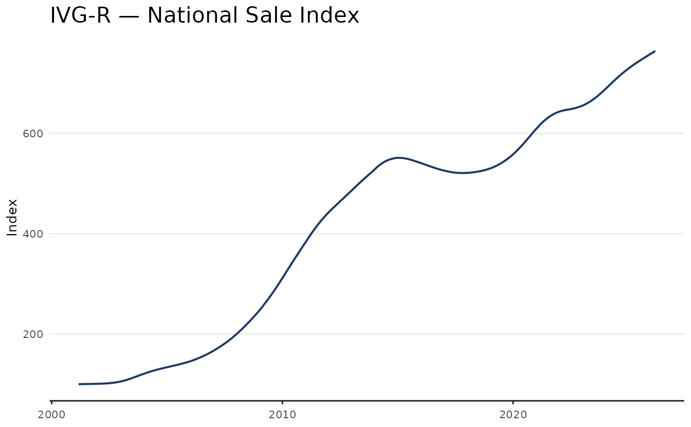

IGMI-R

The IGMI-R (Índice Geral do Mercado Imobiliário Residencial) is published by Abecip/FGV. It uses a hedonic pricing model applied to actual transaction prices, making it the most methodologically rigorous city-level index available. Coverage spans major Brazilian cities from 2014.

igmi <- get_dataset("rppi", "igmi")

glimpse(igmi)
#> Rows: 1,617
#> Columns: 5
#> $ date      <date> 2014-01-01, 2014-01-01, 2014-01-01, 2014-01-01, 2014-01-01,…
#> $ name_muni <chr> "São Paulo", "Rio De Janeiro", "Belo Horizonte", "Fortaleza"…
#> $ index     <dbl> 100.00000, 100.00000, 100.00000, 100.00000, 100.00000, 100.0…
#> $ chg       <dbl> NA, NA, NA, NA, NA, NA, NA, NA, NA, NA, NA, 0.0003654000, 0.…
#> $ acum12m   <dbl> NA, NA, NA, NA, NA, NA, NA, NA, NA, NA, NA, NA, NA, NA, NA, …

main_cities <- c("São Paulo", "Rio De Janeiro", "Belo Horizonte", "Brasília")

subigmi <- igmi |>
  filter(name_muni %in% main_cities)

ggplot(subigmi, aes(date, index, color = name_muni)) +
  geom_line(linewidth = 0.8) +
  labs(
    title = "IGMI-R — Sale Index by City",
    x = NULL,
    y = "Index",
    color = NULL
  ) +
  theme_series()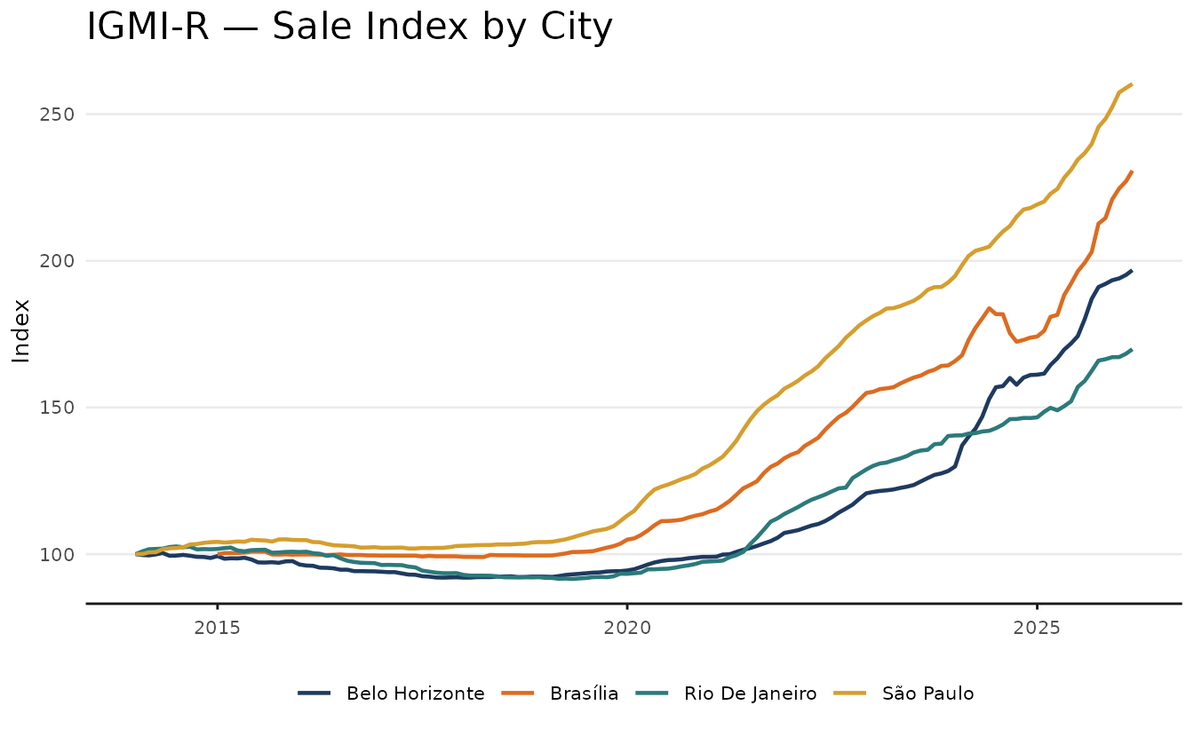

FipeZap (sale)

FipeZap is the broadest RPPI in terms of geographic coverage, with indices for more than 50 cities. It is based on median listing prices rather than transaction prices. Available from 2008 for both residential and commercial markets, with breakdowns by number of bedrooms. Prices are stratified by region and income level, using Census weights, and the final series is smoothed using a 3-month moving average.

Key columns specific to FipeZap:

• market (residential/commercial),
• rent_sale (rent/sale),
• rooms (1, 2, 3, 4+, total),
• variable (index, chg, acum12m, price_m2, yield).

fz <- get_dataset("rppi", table = "fipezap")

glimpse(fz)
#> Rows: 677,160
#> Columns: 7
#> $ date      <date> 2008-01-01, 2008-01-01, 2008-01-01, 2008-01-01, 2008-01-01,…
#> $ name_muni <chr> "Brazil", "Brazil", "Brazil", "Brazil", "Brazil", "Brazil", …
#> $ market    <chr> "residential", "residential", "residential", "residential", …
#> $ rent_sale <chr> "sale", "sale", "sale", "sale", "sale", "sale", "sale", "sal…
#> $ variable  <chr> "index", "index", "index", "index", "index", "chg", "chg", "…
#> $ rooms     <chr> "total", "1", "2", "3", "4", "total", "1", "2", "3", "4", "t…
#> $ value     <dbl> 41.81107, 39.46609, 40.45048, 43.47948, 47.09432, NA, NA, NA…

Working with this dataset requires more complex filtering. For most use cases, however, the main choices are selecting the market (either ‘residential’ or ‘commercial’), rent_sale (either ‘sale’ or ‘rent’), and the desired variable.

subzap <- fz |>
  filter(
    market == "residential",
    rent_sale == "sale",
    rooms == "total",
    variable == "index",
    name_muni %in% main_cities
  )

ggplot(subzap, aes(date, value, color = name_muni)) +
  geom_line(linewidth = 0.8) +
  labs(
    title = "FipeZap — Residential Sale Index",
    x = NULL,
    y = "Index",
    color = NULL
  ) +
  theme_series()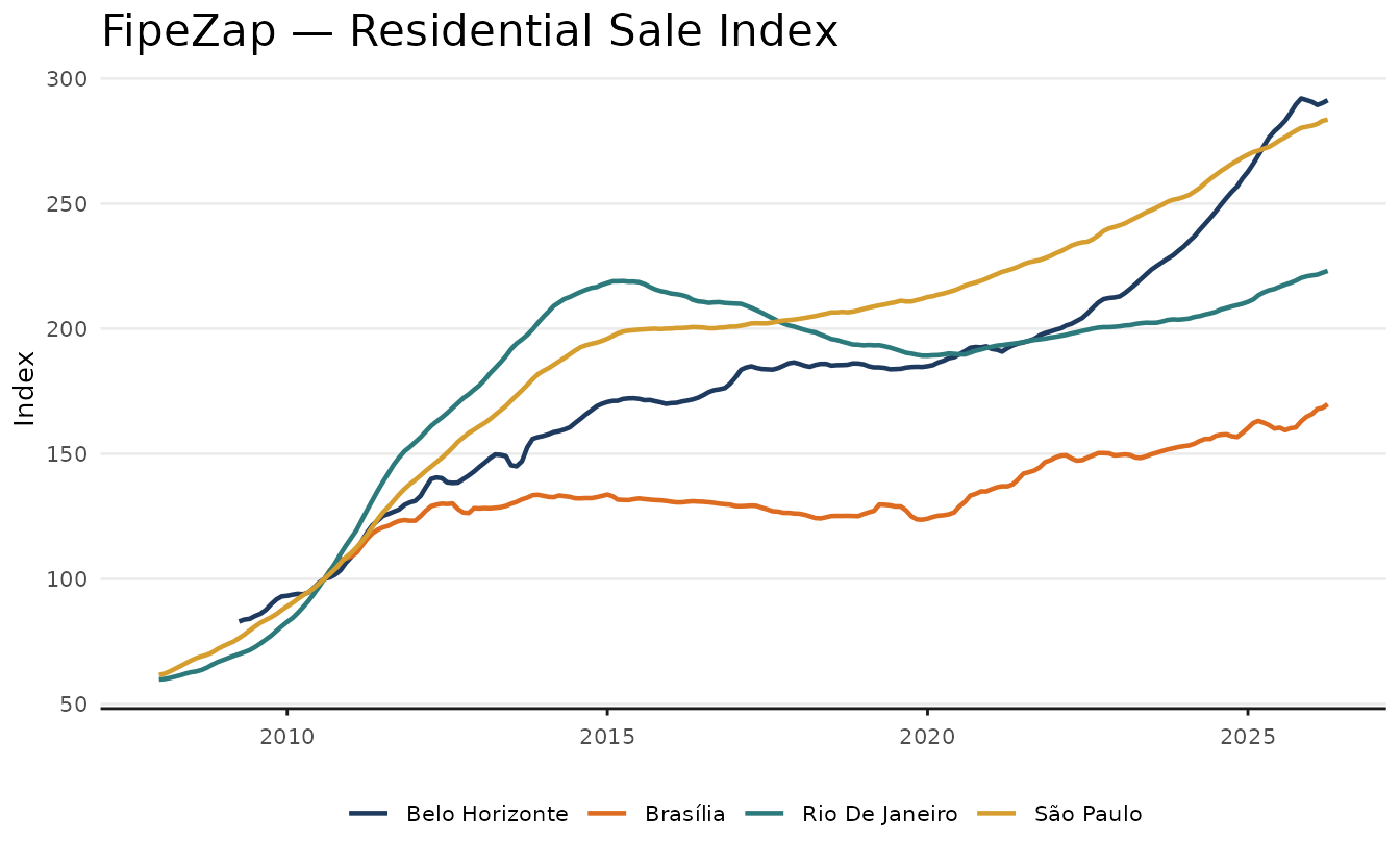

Comparing indices

As mentioned above, the table parameter accepts a "sale" argument, which stacks all available indices into a single tibble.

sale_indices <- get_dataset("rppi", "sale")

glimpse(sale_indices)
#> Rows: 14,458
#> Columns: 6
#> $ source    <chr> "IGMI-R", "IGMI-R", "IGMI-R", "IGMI-R", "IGMI-R", "IGMI-R", …
#> $ date      <date> 2014-01-01, 2014-01-01, 2014-01-01, 2014-01-01, 2014-01-01,…
#> $ name_muni <chr> "São Paulo", "Rio De Janeiro", "Belo Horizonte", "Fortaleza"…
#> $ index     <dbl> 100.00000, 100.00000, 100.00000, 100.00000, 100.00000, 100.0…
#> $ chg       <dbl> NA, NA, NA, NA, NA, NA, NA, NA, NA, NA, NA, 0.0003654000, 0.…
#> $ acum12m   <dbl> NA, NA, NA, NA, NA, NA, NA, NA, NA, NA, NA, NA, NA, NA, NA, …

For convenience, the stacked version of the dataset implicitly only includes rooms == "total" for FipeZap. Also, “Brazil” (spelled with a ‘z’) is listed under name_muni, which shows the nation-wide index, instead of the city specific ones.

The plot shows the three sale indexes at a national level. While there’s some convergence between the indices, there is a growing gap between them in the post-pandemic years. This highlights the importance of choosing the right index for your use case.

comp_index <- sale_indices |>
  filter(name_muni == "Brazil", date >= as.Date("2015-01-01"))

ggplot(comp_index, aes(date, acum12m * 100, color = source)) +
  geom_line(linewidth = 0.7) +
  labs(
    title = "Comparing Sale Indices in Brazil",
    subtitle = "12-month accumulated change (%)",
    y = "%",
    color = NULL
  ) +
  theme_series()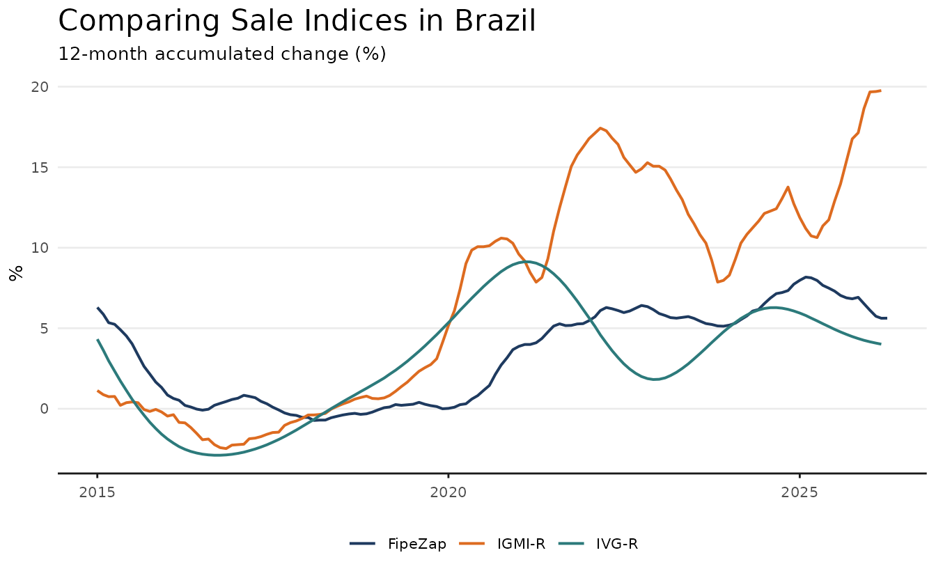

Rent Indices

IVAR

The IVAR (Índice de Variação de Aluguéis Residenciais) is published by FGV and uses a repeat-rent methodology applied to actual rental contracts. It covers major Brazilian cities from 2019 and is available at both city and national level. Notably, the index has no smoothing, making it rather volatile.

ivar <- get_dataset("rppi", table = "ivar")

glimpse(ivar)
#> Rows: 445
#> Columns: 5
#> $ date      <date> 2018-12-01, 2018-12-01, 2018-12-01, 2018-12-01, 2018-12-01,…
#> $ name_muni <chr> NA, "São Paulo", "Rio De Janeiro", "Belo Horizonte", "Porto …
#> $ index     <dbl> 100.000, 100.000, 100.000, 100.000, 100.000, 99.852, 99.731,…
#> $ chg       <dbl> NA, NA, NA, NA, NA, -1.480000e-03, -2.690000e-03, 8.310000e-…
#> $ acum12m   <dbl> NA, NA, NA, NA, NA, NA, NA, NA, NA, NA, NA, NA, NA, NA, NA, …

For the plot, I add a 5-month moving average using the trendseries package.

library(trendseries)

ivar_trend <- ivar |>
  filter(name_muni != "Brazil") |>
  augment_trends(
    value_col = "index",
    group_cols = "name_muni",
    method = "ma",
    window = 5
  )

ggplot(ivar_trend, aes(date, color = name_muni)) +
  geom_line(aes(y = index), lwd = 0.5, alpha = 0.5) +
  geom_line(aes(y = trend_ma), lwd = 0.7) +
  geom_hline(yintercept = 100) +
  scale_x_date(date_breaks = "1 year", date_labels = "%Y") +
  labs(
    title = "IVAR — City Rent Indices",
    subtitle = "Smoothed moving average (5-month window)",
    x = NULL,
    y = "Index"
  ) +
  theme_series()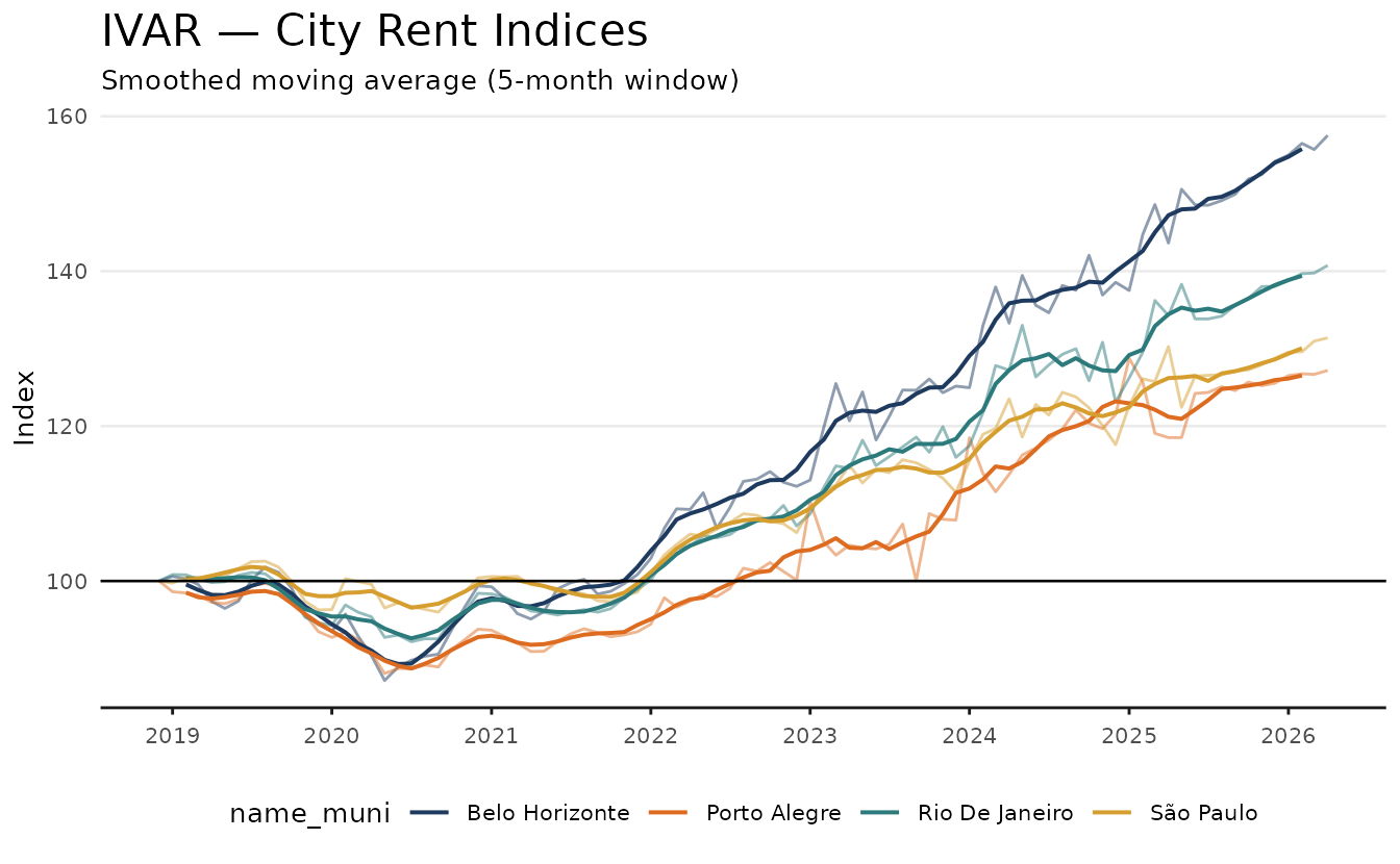

IQA and IQAIW

QuintoAndar published two successive rental indices for São Paulo and Rio de Janeiro. The IQA (2019–mid-2023) was based on median contract prices. In mid-2023 it rebranded to IQAIW (Índice QuintoAndar ImovelWeb) and adopted a hedonic model incorporating both listing and contract prices. The two series are not directly comparable due to the methodology break.

The original IQA compared median contract prices, stratified by region and income level (using Census weights, similar to FipeZap). The IQAIW uses a hedonic model (spatial GAM), double imputation, and a similar Census-based stratification.

Notably, the IQA returns rent prices (R$/m²) rather than an index, so a base-100 normalisation is needed to build an index. For convenience, the distribution includes a simple index based on first available value.

iqa <- get_dataset("rppi", "iqa")
iqaiw <- get_dataset("rppi", "iqaiw")

glimpse(iqaiw)
#> Rows: 1,660
#> Columns: 6
#> $ date      <date> 2019-05-01, 2019-10-01, 2019-11-01, 2019-12-01, 2020-01-01,…
#> $ name_muni <chr> "Belo Horizonte", "Belo Horizonte", "Belo Horizonte", "Belo …
#> $ rooms     <chr> "total", "total", "total", "total", "total", "total", "total…
#> $ index     <dbl> 100.0000, 100.1882, 100.4708, 100.6167, 101.3517, 102.6531, …
#> $ chg       <dbl> NA, 0.003514777, 0.002820158, 0.001452626, 0.007304582, 0.01…
#> $ acum12m   <dbl> NA, NA, NA, NA, NA, NA, NA, NA, 0.07024414, 0.07004492, 0.07…

ggplot(iqa, aes(date, index, color = name_muni)) +
  geom_line(linewidth = 0.7) +
  geom_hline(yintercept = 100) +
  scale_x_date(date_breaks = "1 year", date_labels = "%Y") +
  labs(
    title = "IQA — Rent Index",
    subtitle = "Index (2019/06 = 100)",
    y = "Index",
    color = NULL
  ) +
  theme_series()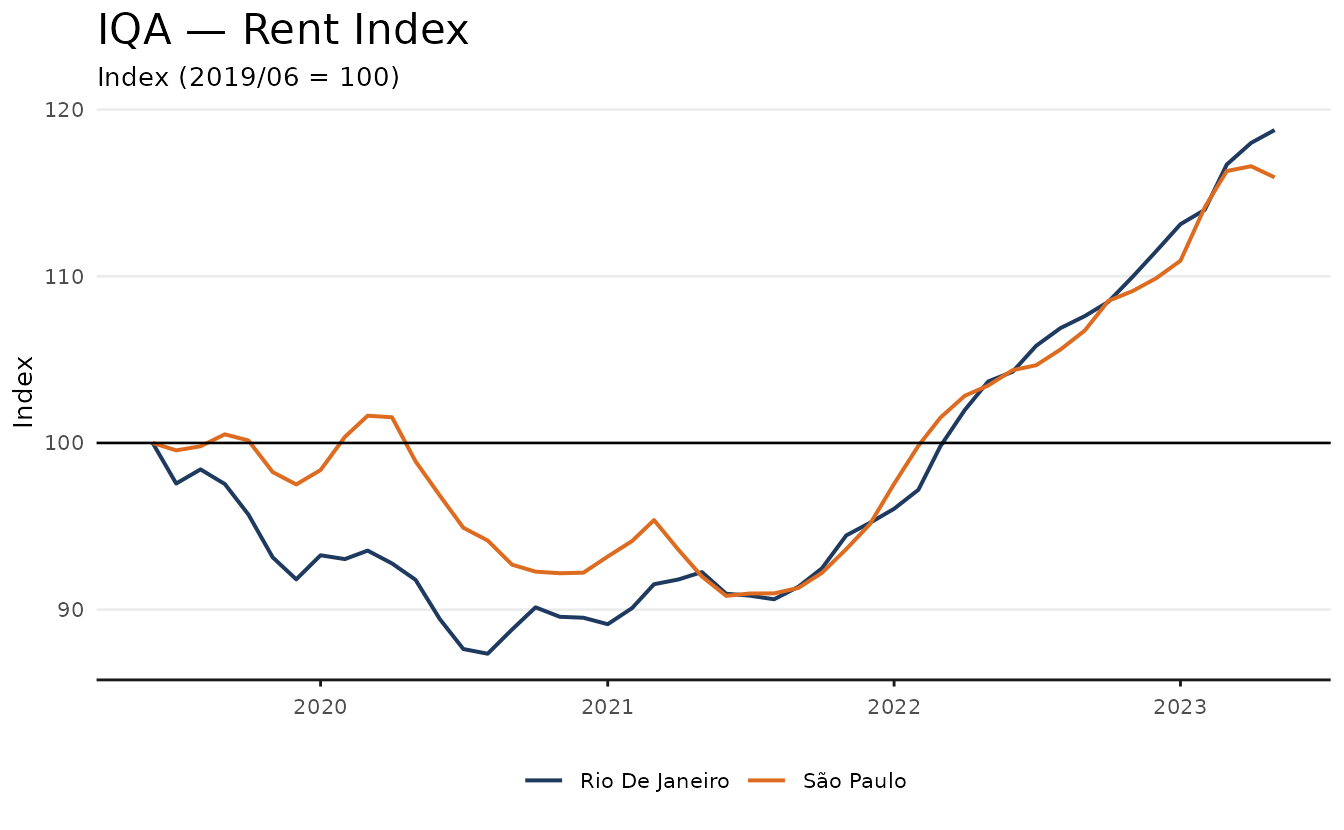

The newer IQAIW index has more cities and, similar to FipeZap, has a bedroom stratification (rooms).

ggplot(
  subset(iqaiw, rooms == "total" & !is.na(acum12m)),
  aes(date, acum12m * 100, color = name_muni)
) +
  geom_line(linewidth = 0.7) +
  scale_x_date(date_breaks = "1 year", date_labels = "%Y") +
  labs(
    title = "IQAIW — Rent Index",
    subtitle = "Accumulated 12-month change (%)",
    y = "%",
    color = NULL
  ) +
  theme_series()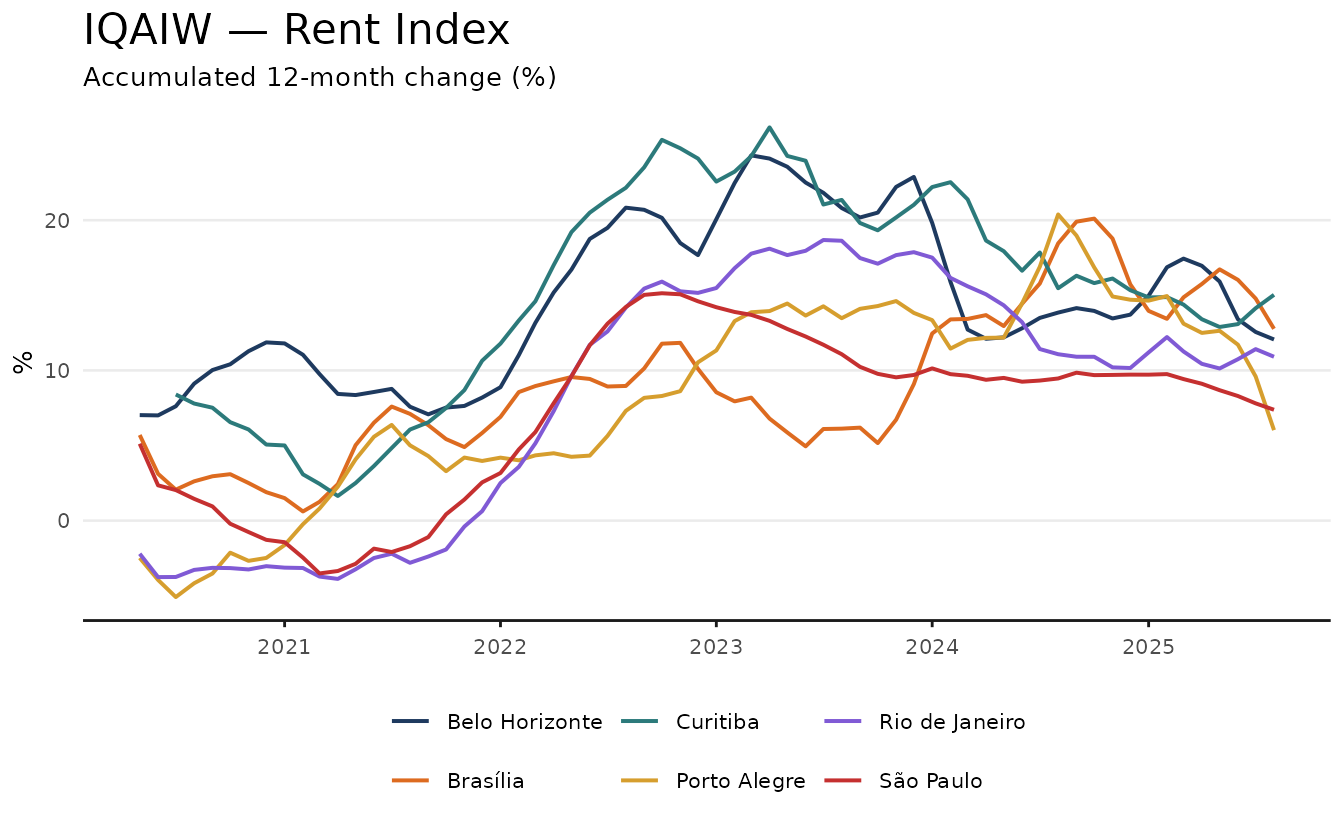

Finally, note that IQAIW is effectively the newer (and improved) version of the older IQA index, which is kept for historical purposes.

quintoandar <- bind_rows(
  list("IQA" = iqa, "IQAIW" = iqaiw),
  .id = "source"
)

quintoandar_spo <- quintoandar |>
  filter(name_muni == "São Paulo", !rooms %in% c("1", "2", "3"))

ggplot(quintoandar_spo, aes(date, index, color = source)) +
  geom_line(linewidth = 0.7) +
  geom_hline(yintercept = 100) +
  scale_x_date(date_breaks = "1 year", date_labels = "%Y") +
  labs(
    title = "QuintoAndar Rent Index — São Paulo",
    subtitle = "IQA (pre-2023) and IQAIW (post-2023) use different methodologies",
    x = NULL,
    y = "Index",
    color = NULL
  ) +
  theme_series()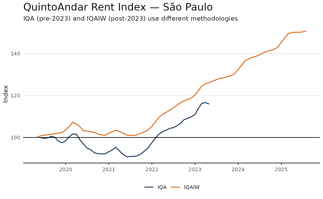

FipeZap (rent)

FipeZap provides the broadest geographic coverage for rental indices, but is based on median listing prices rather than contracts. The example below shows the 12-month accumulated change across cities with complete data from 2021.

fz <- get_dataset("rppi", table = "fipezap")

glimpse(fz)
#> Rows: 677,160
#> Columns: 7
#> $ date      <date> 2008-01-01, 2008-01-01, 2008-01-01, 2008-01-01, 2008-01-01,…
#> $ name_muni <chr> "Brazil", "Brazil", "Brazil", "Brazil", "Brazil", "Brazil", …
#> $ market    <chr> "residential", "residential", "residential", "residential", …
#> $ rent_sale <chr> "sale", "sale", "sale", "sale", "sale", "sale", "sale", "sal…
#> $ variable  <chr> "index", "index", "index", "index", "index", "chg", "chg", "…
#> $ rooms     <chr> "total", "1", "2", "3", "4", "total", "1", "2", "3", "4", "t…
#> $ value     <dbl> 41.81107, 39.46609, 40.45048, 43.47948, 47.09432, NA, NA, NA…

Note that this table is the same as the one used in the previous sales example.

fz_rent <- fz |>
  filter(
    market == "residential",
    rent_sale == "rent",
    rooms == "total",
    variable == "acum12m",
    date >= as.Date("2019-01-01")
  )

sel_cities <- fz_rent |>
  filter(date == "2019-01-01", !is.na(value)) |>
  pull(name_muni)

The plot emphasizes the main strength of FipeZap’s index: its broad geographic coverage.

ggplot(subset(fz_rent, name_muni %in% sel_cities), aes(date, value * 100)) +
  geom_line(linewidth = 0.7, color = color_palette[1]) +
  geom_hline(yintercept = 0) +
  facet_wrap(vars(name_muni)) +
  labs(
    title = "FipeZap — 12-month Rent Change by City",
    x = NULL,
    y = "Accumulated 12-month change (%)"
  ) +
  theme_series()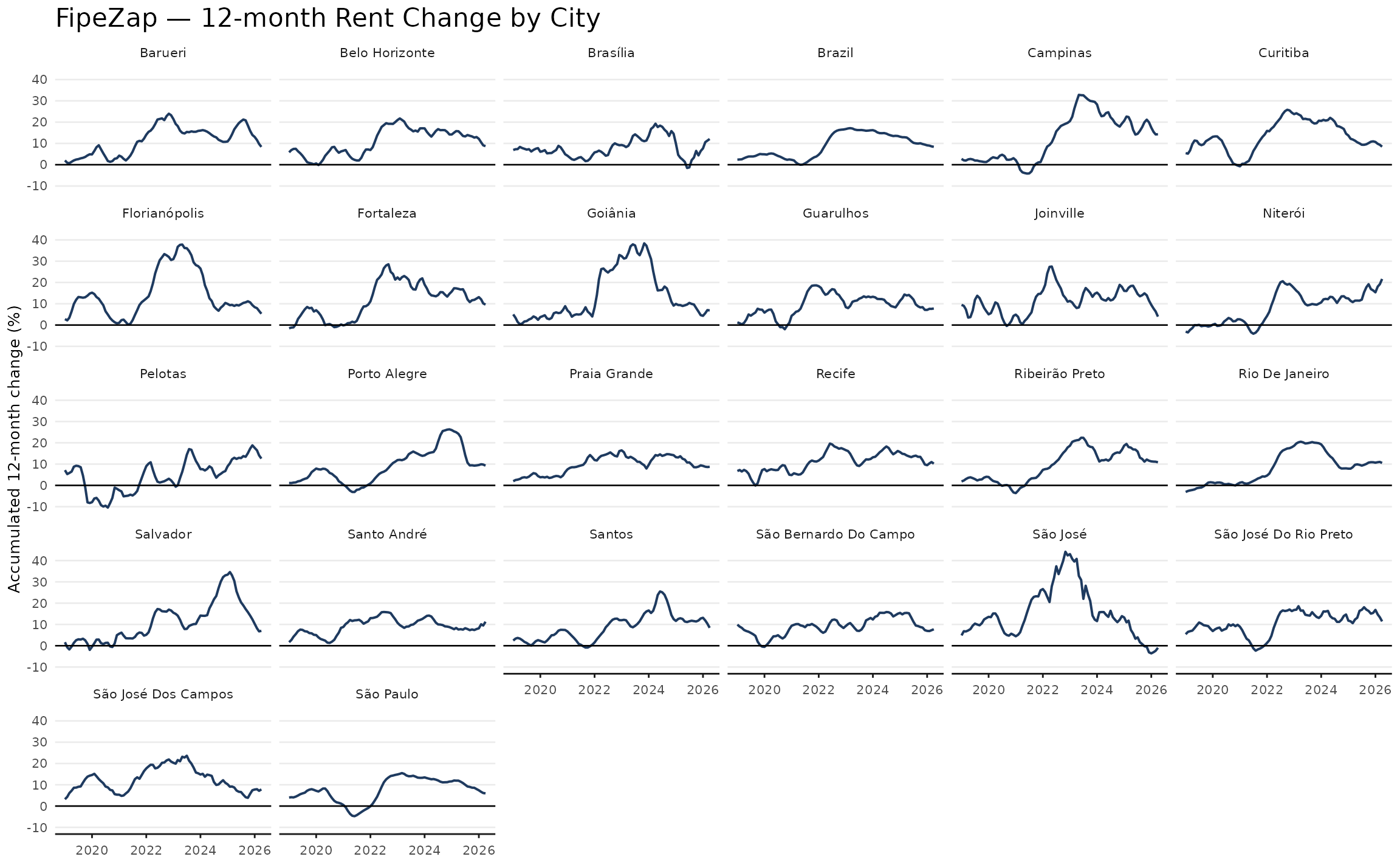

SECOVI-SP

SECOVI-SP publishes a residential rent index for the city of São Paulo. The series tracks median contract prices for residential leases and is available from 2008, making it one of the longest rent series for a single Brazilian city.

secovi <- get_dataset("rppi", "secovi_sp")

glimpse(secovi)
#> Rows: 236
#> Columns: 5
#> $ date      <date> 2004-12-01, 2005-01-01, 2005-02-01, 2005-03-01, 2005-04-01,…
#> $ name_muni <chr> "São Paulo", "São Paulo", "São Paulo", "São Paulo", "São Pau…
#> $ index     <dbl> 100.000, 100.500, 100.802, 101.003, 101.104, 101.306, 101.71…
#> $ chg       <dbl> NA, 0.0050000000, 0.0030049751, 0.0019940081, 0.0009999703, …
#> $ acum12m   <dbl> NA, NA, NA, NA, NA, NA, NA, NA, NA, NA, NA, NA, 0.04176000, …

ggplot(secovi, aes(date, acum12m * 100)) +
  geom_line(color = color_palette[1], linewidth = 0.7) +
  geom_hline(yintercept = 0) +
  scale_x_date(date_breaks = "2 years", date_labels = "%Y") +
  labs(
    title = "SECOVI-SP — Residential Rent Index",
    subtitle = "12-month accumulated change (%)",
    x = NULL,
    y = "%"
  ) +
  theme_series()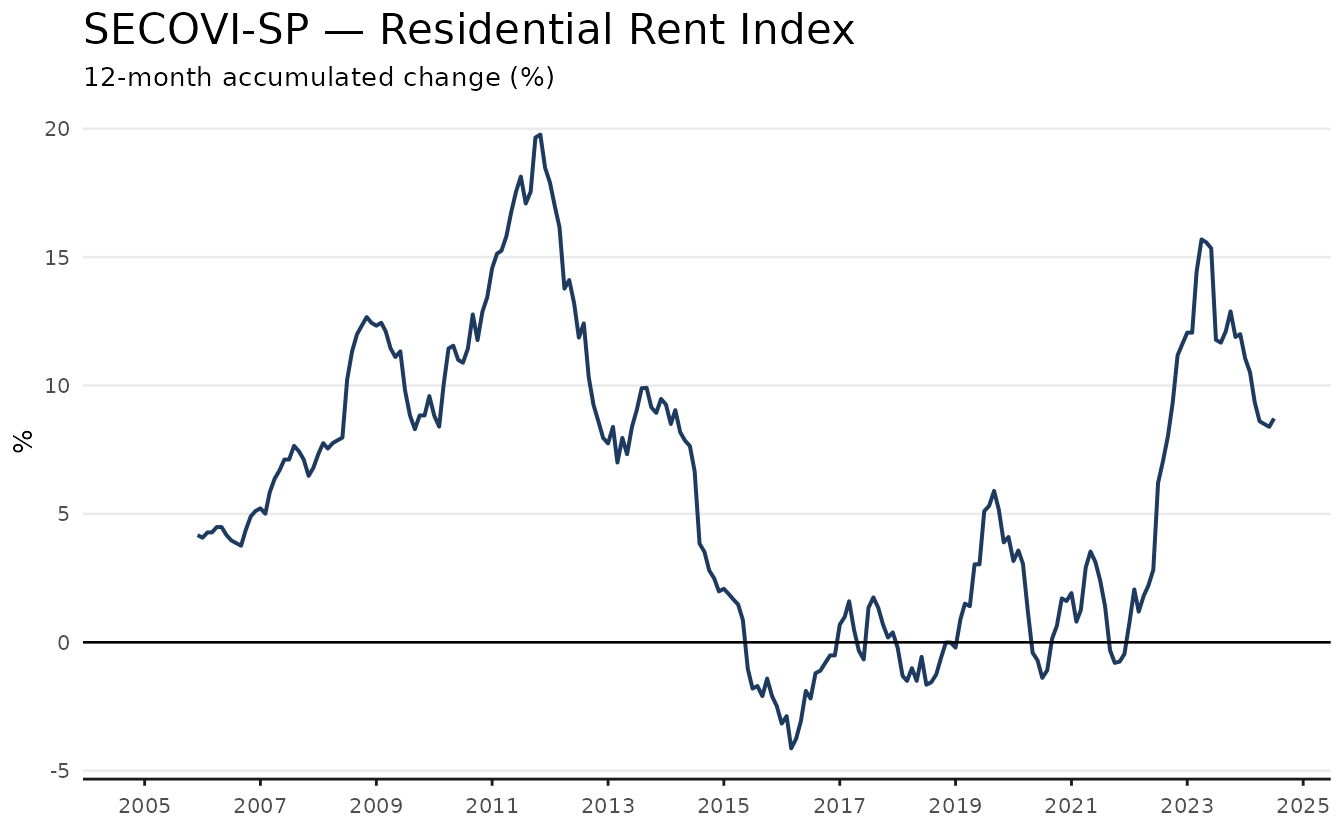

Comparing Indices

Stacked tables

The "sale" and "rent" tables stack all available indices into a single data frame, making cross-source comparisons straightforward.

rent_indices <- get_dataset("rppi", "rent")

rent_indices_comp <- rent_indices |>
  filter(
    name_muni %in% c("São Paulo", "Rio de Janeiro"),
    date >= as.Date("2019-01-01")
  )

ggplot(rent_indices_comp, aes(date, acum12m, color = source)) +
  geom_line(linewidth = 0.7) +
  geom_hline(yintercept = 0) +
  facet_wrap(vars(name_muni)) +
  scale_x_date(date_breaks = "1 year", date_labels = "%Y") +
  labs(
    title = "Rent Indices — São Paulo and Rio de Janeiro",
    subtitle = "12-month accumulated change",
    y = "Accumulated change",
    color = NULL
  ) +
  theme_series()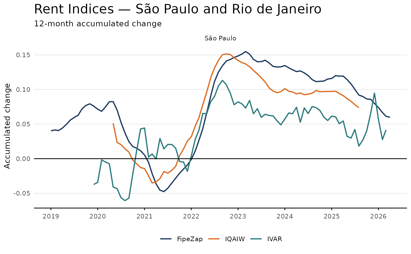

Normalising to a common base

Each index has its own base period, so normalisation is required before comparing levels. The example below rebases all national sale indices to January 2018 = 100.

sales <- get_dataset("rppi", "sale")

national <- sales |>
  filter(
    name_muni == "Brazil",
    date >= as.Date("2018-01-01"),
    date <= as.Date("2023-12-01")
  )

national_rebased <- national |>
  mutate(
    index_rebased = index / first(index) * 100,
    .by = source
  )

total_growth <- national_rebased |>
  summarise(
    growth = last(index_rebased) - first(index_rebased),
    date = last(date),
    index_rebased = last(index_rebased),
    .by = source
  ) |>
  mutate(label = sprintf("%s:\n+%.1f%%", source, growth))

ggplot(national_rebased, aes(date, index_rebased, color = source)) +
  geom_line(linewidth = 0.8) +
  geom_hline(yintercept = 100) +
  geom_label(
    data = total_growth,
    aes(label = label),
    hjust = 0,
    nudge_x = 30,
    nudge_y = c(-5, 10, -5),
    show.legend = FALSE,
    size = 3
  ) +
  scale_x_date(
    date_breaks = "1 year",
    date_labels = "%Y",
    expand = expansion(mult = c(0, 0.125))
  ) +
  labs(
    title = "Brazil National Sale Indices — Rebased to Jan 2018",
    x = NULL,
    y = "Index (Jan 2018 = 100)",
    color = NULL
  ) +
  theme_series()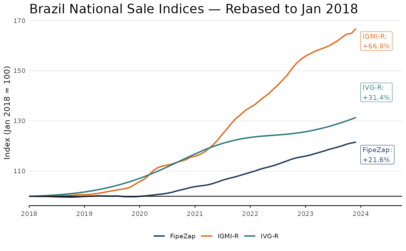

International: BIS

The BIS dataset provides quarterly residential property price indices for 60+ countries, enabling Brazil to be placed in international context.

bis <- get_dataset("rppi_bis")

bis_sub <- bis |>
  filter(
    ref_area_name %in% c("Brazil", "United States", "Germany", "Japan"),
    is_nominal == 0,
    unit == "index",
    date >= as.Date("2000-01-01")
  )

ggplot(bis_sub, aes(date, value, color = ref_area_name)) +
  geom_line(linewidth = 0.8) +
  geom_hline(yintercept = 100, linetype = "dashed", alpha = 0.4) +
  labs(
    title = "Real Residential Property Prices",
    subtitle = "BIS, index 2010 = 100",
    x = NULL,
    y = "Index",
    color = NULL
  ) +
  theme_series()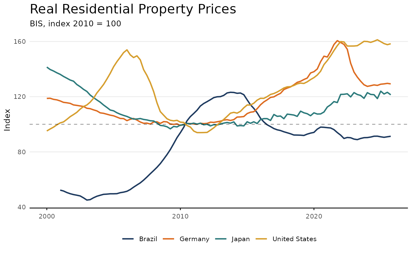

Index Reference

Index	Source	Coverage	Methodology	From
IVG-R	BCB	National	Median appraisal prices, HP-filtered	2001
IGMI-R	ABECIP/FGV	Major cities	Hedonic (transaction prices)	2014
FipeZap	FIPE/ZAP	50 cities	Median listing prices	2008
IVAR	FGV	Major cities + national	Repeat-rent (contracts)	2019
IQA	QuintoAndar	São Paulo, Rio	Median contract prices	2019
IQAIW	QuintoAndar	São Paulo, Rio	Hedonic (listing + contracts)	2023
Secovi-SP	SECOVI-SP	São Paulo	Median prices (transactions)	2008